After much anticipation, we have finally got to the topic that I
keep on mentioning, but never explain – interrupts! Interrupts are
probably the single most important concept that make every electronic
device work as it does. If interrupts didn’t exist, your electronic
devices wouldn’t be as responsive, fast and efficient as they are. They
are the source for all types of timers and ticks and integrated into
most peripherals. Every CPU has interrupt capabilities, although the
capabilities vary widely. Interrupts are sometimes neglected because its
‘easier’ to poll than implement interrupts but its generally considered
poor design. So what are interrupts? They are really just a way for the
hardware to signal the software that some event has occurred. Each
event has an entry in what is called the interrupt vector table – a
table of pointers to functions stored in memory (either flash or RAM),
which the CPU will jump to automatically when the interrupt fires. These
functions are called interrupt service routines (ISR), and though some
may be included as part of the compiler libraries, most need to be
implemented by the programmer. Interrupt service routines must be as
quick and efficient as possible, so as to not stall the software which
was executing. They must also be efficient with the stack. In operating
system environments, interrupt handlers may operate on a separate
[software] stack which is much smaller than a typical process or thread
stack. Also, no blocking calls should be made. Taking too long in the
ISR can result in lost data or events. Interrupts have attributes that
may or may be programmable, depending on the architecture and the
device. In this lesson, we will learn about the different types of
interrupts, their attributes, how to implement them, what happens when
an interrupt fires, and how they are used in real world applications.
The generic interrupt vector table is available in table 2-1 of the
family reference manual, while device specific vectors are defined in
table 5 of the datasheet.
Most interrupts can be enabled or disabled by software. Typically
there is a register that will perform the function globally for all
interrupts or groups of interrupts, and then additional registers for
individual interrupts. Disabling an interrupt is often referred to as
‘masking’ the interrupt. Interrupts are almost always accompanied by a
status or flag register which the software can read to determine if a
specific interrupt has fired. This is required because sometimes many
physical interrupts are connected to the same interrupt request (IRQ) –
the signal to the CPU. The flag is required because the interrupt line
may only be active for a very short amount of time and the software may
not respond fast enough. The flag ensures the the state of the interrupt
is stored somewhere until it is read and cleared by the software. It is
also often used to acknowledge and clear the interrupt, as is the case
with the MSP430. Enabling and disabling interrupts in the MSP430 at a
global level is done through the status register. We have not looked in
detail at the contents of the status register, so lets do that now.
As mentioned above, GIE is the field used to enable or disable
maskable interrupts on the device. The compiler provides intrinsic
functions to do this in C, __enable_interrupts and __disable_interrupts.
Maskable interrupts are disabled by default on reset, so the software
must enable them to use them. Not all interrupts can be disabled. These
are called non-maskable interrupts, or NMI. There are usually some
interrupts on a device that are reserved as NMIs. NMIs are typically
critical errors to which the software must respond and handle in order
to continue execution. The MSP430 has three NMIs.
Sometimes these types of interrupts are referred to as exceptions.
Exceptions can also be raised due to some non-recoverable fault. It is a
similar concept to a software exception, but implemented in hardware.
On the MSP430, there is one non-recoverable exception, the illegal
instruction fetch, which causes a reset. On some architectures, this
exception can be handled and the handler may increment the program
counter to the next address to try and skip over it. Other examples of
exceptions which exist on other architectures are the divide by zero and
invalid memory access. Although not documented as an exception, the
MSP430 does source the reset vector if attempting to execute from an
invalid memory space such as an address not in RAM or flash.
One very common use for interrupts is to detect changes in GPIO
inputs. Stemming from our push button code which has to poll the P1IN
register, enabling an interrupt on a GPIO would allow the hardware to
signal the software when the input has changed values. Not all GPIOs are
interrupt capable, so remember to check in the device datasheet when
choosing which pin to connect it to. GPIO interrupts have their own
subset of properties. The first property is the active signal level –
either active high or active low. Active high means that the signal is
interpreted as active when the line is high (a positive voltage), while
active low means the signal is interpreted as active when the line is
low (0V or ground). However, the second property, edge vs level based
(also known as edge or level triggered interrupts), defines when the
interrupt actually fires. Edge based interrupts will only fire once as
the state of the line transitions from the inactive level to the active
level. Level based interrupts will fire continuously while the input is
at the active level. In order to handle a level based interrupt, the ISR
should mask it so that it does not fire continuously and effectively
stall the CPU. Once the source of the interrupt is cleared, the
interrupt may be enabled so it can fire again. Level based interrupts
are sometimes used to perform handshaking between the source of the
interrupt and the software handling it. The software would enter the
ISR, check the status of the source of the interrupt to determine
exactly what caused the interrupt (remember multiple sources per IRQ),
and then clear source condition and the flag. If the interrupt condition
is successfully cleared, the line will return to the inactive state and
the software will continue on. Otherwise, the line will remain active
and the interrupt would fire again. The MSP430 only supports edge
based interrupts.
Another important attribute of interrupts is the priority. Interrupt
priorities determine which interrupt service routine will be called
first if two interrupts fire at the same time. Depending on the
interrupt controller, some interrupt priorities may be configurable by
software. The MSP430 does not support this, all interrupts have a fixed
priority. The interrupt priorities on the MSP430 are in descending order
from highest address in the vector table to the lowest. One important
concept related to interrupt priorities is interrupt nesting. If one
interrupt fires and the ISR is invoked, and while in the ISR another
interrupt of a high priority fires, the executing ISR may be interrupted
by the higher priority one. Once the higher priority ISR has completed,
the lower priority ISR is then allowed to complete. In the case of the
MSP430, nesting is not dependant on the priority. Any priority interrupt
will be serviced immediately if nested interrupts are enabled. Nesting
interrupts is an advanced topic an will not be enabled for this
tutorial. If an interrupt fires while an ISR is executing, it will be
serviced only once the ISR is complete.
The reset vector is the single most important interrupt available.
Without it, code would never begin executing. The compiler [typically]
automatically populates the reset vector with the address of the entry
point of the .text section, i.e. the __start function. When a device is
powered on or the reset pin is toggled, the reset vector is sourced and
the CPU jumps to the address it contains. Going back to the linker
script from last lesson, the table of memory regions has a region
defined for each interrupt vector. A region called RESETVEC is located
at 0xFFFE, defined with a size of 2 bytes. Then a section called
__reset_vector is created and assigned to this memory location. The data
allocated to this section will be the address of the reset vector ISR.
To show that the reset vector is assigned the start-up code, the
following command can be used:
Passing the argument -D to objdump is similar to -S, but it dumps the
disassembly for all sections rather than just the .text section as -S
does. This is required because as mentioned above, the reset vector is
part of its own section, not the .text. The output of this command will
look like this:
The first couple lines of code are all we are interested in. We can
see that the first section in the output is the reset vector. In it
there is only one label: ‘__msp430_resetvec_hook’. At this label there
is 2 bytes of data allocated with the value of 0xc010 (keep in mind the
endianess). Search for 0xc010, and you will see that this is the address
of __start, the entry point. Therefore as expected, when sourced the
reset vector shall cause the CPU to jump to the start-up code.
The watchdog is another very important interrupt. It is actually a
whole module which is implemented as part of almost every MCU, SoC, etc…
The purpose of the watchdog is to ensure that the software is running
and had not stopped, crashed or otherwise been suspended. It is very
rare that you find an embedded system without a watchdog. If implemented
correctly in both hardware and software, the device should never stall
indefinitely. Once enabling the watchdog, the software must pet it
periodically with an interval less than its timeout. Failure to do so
will result in the watchdog resetting the device. In the case of the
MSP430, the watchdog interrupt is the same as the reset vector, so a
watchdog interrupt will reset the device. Some devices have more
complex watchdogs which generate an intermediate interrupt to allow the
software to perform any logging or cleanup operations before resetting.
The MSP430 watchdog module does not support this, but it has an
additional interesting feature – it can be configured as a regular
16-bit timer. This could be useful if an additional timer if needed. We
will be configuring the watchdog in watchdog mode because it is
important to understand how to setup the module and how it should be
maintained by the software. The watchdog is configured and monitored
through the 16-bit register WDTCTL and two additional registers,
interrupt enable 1 (IE1) and interrupt flag 1 (IFG1).
The blank fields of IE1 and IFG1 registers are determined by the
specific device and will be covered as needed. Now lets use what we have
learned to disable and enable the watchdog timer in our existing code
and watch the device reset. Below is a set of a set of functions to
perform these actions.
The first function disables the watchdog exactly as we do currently
in our main function. The _disable_watchdog function should be called
right at the beginning of your code in order to avoid accidentally
generating a reset when modifying the configuration. You can go ahead
and replace the existing watchdog code in main with a call to this
function. In the enable function, the watchdog timer interrupt flag is
read and cleared if required. If the flag is set, some action could be
performed such as logging the number of watchdog resets but we have no
need at this time. Then _watchdog_pet is called. Petting the watchdog
will effectively enable it as well. Only two fields are set in the
WDTCTL register, the password field WTDPW and the clear counter bit
WDTCNTCL. The watchdog will be enabled since the WDTHOLD bit is cleared.
The timeout of the watchdog timer is determined by the clock source
select bit WDTSSEL and the interval select field WDTISx. This means the
watchdog timer will source its clock from ACLK and expire after 32768
clock cycles. In
we
did not configure ACLK but now we must. ACLK should be configured to be
sourced from VLOCLK, which is approximately 12kHz. If we tried to
source it from MCLK or SMCLK, the timeout would be too short for the
delay required by the blinking LED. To configure ACLK, in main we must
add a new line under the clock configuration.
Since the interval selector is set to 32768 clock cycles at 12kHz,
the timeout of the watchdog will be 2.73s. Therefore the watchdog must
be pet at least every 2.73s. Since our loop delay 500ms each iteration,
we are within the requirements of the watchdog. Now lets see that the
watchdog actually fires and resets the device. Call the watchdog enable
function right after detecting the button press.
Typically you would want to enable the watchdog as soon as possible,
especially before any infinite loops. In case this I want you to control
when the watchdog is enabled so that you can see when it resets.
Compile the code and program it to the device. Set a breakpoint at the
new function _watchdog_enable (use nm to find the address). Run the code
and press the button. When it stops at the breakpoint run it and press
the button again. The breakpoint will be hit again. This shows that the
device is restarting. To verify that it is because of the watchdog, we
can read the register IFG1 and see if WDTIFG is set. IFG1 is located at
address 0x02 as indicated in both the datasheet and the family reference
manual. Read this address using the md command. You should see the
following:
The value of the IE1 is 0x7, therefore the WDTIFG bit is set. It is
important to note that the other bits which are set are defined by the
device specific implementation which can be found in the datasheet. They
are PORIFG (bit 2), the power on reset interrupt flag, and OFIFG (bit
1), the oscillator fault interrupt flag. These two bits are set because
that is their default value after reset. Now we will pet the watchdog to
prevent it from resetting the device. Call _watchdog_pet inside the
while loop that toggles the LED.
Compile the code and program the board. Press the button to enable
the watchdog and notice that now the board does not reset (note the
address of the breakpoint will need to be adjusted since you added new
code). And that’s basically how to pet a watchdog. As we add more code
to our project, we will see how the watchdog needs to be managed to
ensure that it only trips if there is a failure and not because the code
is waiting for some input.
Now we will get into the details of interrupt handling on the MSP430.
When an interrupt fires, a few things have to happen before entering
the ISR:
Now the CPU can begin executing the ISR. All of this happens in
hardware, no software is involved so you will never see this in code. It
can be inspected by using the debugger however, and we will see this
shortly. The time starting from when the interrupt is triggered to the
time when the ISR is invoked, is called the interrupt latency. In the
case of the MSP430, the interrupt latency is 6 clock cycles.
The ISR has some responsibilities of its own before executing the
application code. If written in C, this is taken care of by the
compiler. In assembly it must be implemented manually. To see how this
works, we are going to create an interrupt service routine in C to
detect the button press. Unfortunately, there is no way defined by the C
programming language on how to declare an interrupt handler, it is left
up to the compiler. Therefore what you will learn is only applicable
for gcc and may look slightly different on other compilers. To declare
an ISR in gcc you must use the ‘attributes’ feature. Attributes provide
additional functionality which are non-standard. When possible, using
attributes should be avoided so that the code is compiler agnostic (read
– portable from one compiler to another). There are some attributes
which are common across compilers and it is often considered good
practice to define them as macros in a separate header file (often name
compiler.h) which uses hash defines to compile the macros relevant for
that compiler. To declare the interrupt service routine, we first need
to figure out which interrupt we are going to write an ISR for. On the
MSP430, each IO port is assigned an interrupt. It is up to the software
to determine which pin on the port was the source. So how so do we refer
to this interrupt? Open the msp430g2553.h header file and search for
‘PORT1_VECTOR’. You will find the list of interrupt vectors for this
device. The desired vector should be passed to the interrupt attribute.
It tells the compiler in which section to place the address of your ISR.
Therefore, our empty function declaration would look like this:
ISRs must have a return type of void and have no arguments. Lets see
what has been generated using the the objdump command from earlier to
disassemble the code.
We can see that a new section has been added called
__interrupt_vector_3. To understand this we need to go to the datasheet
and find the address of the interrupt vector for port 1 (since our
button is connected to P1.3). The vector is located at address 0xFFE4.
In the linker script memory region table, this address is part of the
region VECT3. In the sections table, we can see that the section
__interrupt_vector_3 is loaded into region VECT3. This means that when
passing vector 3 (which PORT1_VECTOR is defined as) to the interrupt
attribute, the compiler will place the address of that function at
0xFFE4. From the objdump output, we can see the value at 0xFFE4 is
0xC278. Search in the rest of the file for this address and you will
find that it is in fact our function port1_isr. Currently the function
is empty, so lets go back and fill it in. In order to start or stop the
the blinking LED using the push button, we will need some sort of signal
between our main function and the ISR. We will use a simple variable
which will be toggled by the ISR.
For some of you volatile may be a new keyword that you have not used
before. Volatile tells the compiler that the value of that variable may
be changed at any time, without any nearby code changing it. This is the
case for an ISR. The compiler cannot know when the ISR is going to
fire, so every time the variable is accessed, it absolutely must read
the value from memory. This is required because compilers are smart, and
if they determine that nothing nearby can change the value, it may
optimize the code in such a way that the value will not be read. In this
case, that change will occur in the ISR so it must be read every single
time. Next we have to introduce a few new registers, PxIES, PxIE and
PxIFG (where ‘x’ is the port number). All three of these register follow
the same bit-to-pin convention as the other port configuration
registers we have previously discussed. The latter two are similar to
IE1 and IE2, they are the port interrupt enable and port interrupt flag
registers. PxIES is the interrupt edge select registers where a bit set
to 0 signals an interrupt for a low-to-high transition (active-high) and
a bit set to 1 signals an interrupt on a high-to-low transition
(active-low). Now that we have covered how to configure the interrupts,
let’s modify our code to use it. First, instead of waiting in a while
loop to start the LED blinking, let the interrupt handler enable it, so
remove the first while loop. The interrupt should be configured before
the watchdog is enabled. Since the button is on P1.3 and it is
pulled-up, we want to set the interrupt to occur on a high-to-low
transition so bit 3 in PIES and P1IE should be set high. Finally, enable
interrupts using the intrinsic function __enable_interrupt. In the
while loop, modify the code to only blink the LED when _blink_enable is
non-zero. Your code should look something like this:
Now for the ISR. Since one interrupt is sourced for all the pins on
the port, the ISR should check that P1.3 was really the source of the
interrupt. To do so, we must read bit 3 of P1IFG and it is high, toggle
_blink_enable and then return.
All of these changes are available in the latest lesson_6 tag on
github. Recompile the code and use objdump to inspect the ISR. The
address of the ISR can be found by looking at the contents of the
__interrupt_vector_3 section from objdump as we did for the reset
vector.
The first operation is to push R12 onto the stack. R12 is the
register the compiler is going to use to toggle the variable
_blink_enable. It must ensure that the previous value is stored because
it may be used by the function which has been interrupted. If the ISR
clobbers the register value, when the interrupted function continues
execution, the register would have the wrong value. This applies to all
registers and it is up to the compiler to determine which registers are
used by the ISR and thus must be pushed on the stack. In this case only
R12 is being used, so the most efficient implementation is to push only
R12. Now that R12 is free to use, it can be used to check the value of
P1IFG and ensure the flag is set. Then in order to acknowledge the
interrupt so it doesn’t fire again, the flag must be cleared. The
address of P1IFG (0x23) is loaded into R12 and bit 3 is cleared. Finally
the address of our variable _blink_enable is loaded into the register
and the value is XOR’d with 0x1. The stack is popped back into R12 to
restore the initial value before returning. To return from an interrupt,
the RETI pseudo-instruction is used. RETI, which stands from return
from interrupt, tells the CPU to pop off the SR and PC values back into
their respective registers. Now that all the registers are exactly as
they were before the interrupt fired, the flow of execution continues on
as if nothing happened. Now program the device and run the new code.
The LED will begin blinking once the button is pressed, and pressing the
button again will toggle the blinking on or off. Set a breakpoint at
port1_isr. When the button is pressed the CPU will be stopped at
the ISR. The stack pointer is set to ~0x3f4 (depending where exactly the
code was interrupted) and dumping the memory at this location, we can
see the result of entering the ISR.
The first 2 bytes on the stack will be the SR. The value of the
status register stored in the stack will be different from that
currently dumped by mspdebug since it is cleared by the hardware. The
next 2 bytes will be the PC, in this case 0xc2b0. Using objdump to view
the code at this address, we can see that the CPU was interrupted right
at the end of _watchdog_pet, which is called within the while loop, as
expected. Your values may differ slightly depending where exactly the PC
was when you pressed the button. What we really have experienced here
is something commonly known as a context switch. It is the foundation of
all software, not just embedded systems. Almost every operating system
uses context switching to some extent, usually triggered by an interval
timer firing an interrupt periodically. This is what allows you have to
many threads and processes running on just one CPU. Its the illusion of
parallel operation through the use of extremely fast context changes
many times per second. The definition of the context is dependent on the
architecture. In the case of the MSP430, it is all the main CPU
registers we have discussed in the last lesson. When the ISR fires, we
have to save all of these registers that could be modified so when the
interrupt completes, the context can be restored. A context switch of a
thread or task (synonymous terms) would have to save all the registers
on its stack before restoring the registers for the task about to run.
There is some really interesting stuff here, and this is only an
introduction. We will not be creating a multi-threaded system since that
is way beyond the scope of this course, but interrupts are a form of
context switch so it is important to understand how powerful and
important they really are in embedded systems.
In this lesson we are going to go on a bit of a tangent and take
care of some housekeeping duties to accommodate our growing code base.
Until now, we have been writing all the code in a single file, and
compiling by invoking gcc on the command line. Clearly neither of the
are scalable nor feasible solutions for for a full embedded development
project. We need to separate our code into logical modules, create
header files will APIs to interface with them and introduce a new tool
that will help us maintain our build system and environment. This tool
is called ‘make’. Make is GNU utility which is the de-facto standard in
the open source community for managing build environments. Most IDEs
(notably Eclipse and its derivatives) use make or a form a make to
manage the build. To the user its looks like a series of files in a
folder which get compiled when you press build, but under the hood a
series of scripts are being invoked by make which does all the real
work. Make does several things which we will look at in this tutorial.
First, it allows you to defined compiles rules, so instead of invoking
gcc from the command line manually, you can script it so it passes in
the files and the compiler options automatically. It allows you to
better organize your code into directories, for example, one directory
for source files, one for header files and another one for the build
output. And finally, it can be used to track dependencies between files –
in other words, not all files need to be recompiled every time and this
tool will determine which files need to be compiled with the help of
some rules we will add to the script. Make is an extremely powerful
tool, so we will just scratch the surface in this tutorial to get us
started. But before we jump into make, we must start by cleaning up our
code.
Reorganizing the code
As you know, all the code we have written is currently in one file,
main.c. For such a small project, this is possibly acceptable. However
for any real project functions should be divided into modules with well
defined APIs in header files. Also, we do not want to have a flat
directory structure so we must organize the code into directories. The
directory structure we will start with is going to be simple yet
expandable. We will create three directories:
- src: where all the source files go
- include: where all the header files go
- build: where all the output files go
Create the new directories now.
cd ~/msp430_launchpad
mkdir src
mkdir include
The build directory will actually be generated by the build
automatically, so we don’t have to create it manually. You rarely check
in the built objects or binary files into the SCM (git) so the build
directory should be added to the .gitignore file. Open the .gitignore
file (a period in front of a filename means it is hidden in Linux – you
can see it with the command ls -al) and on the next line after ‘*.out’
add ‘build/’, save and close. You will not see the new directories under
git status until there is a file in them as git ignores empty
directories. Move main.c into the src/ directory.
mv main.c src
Open main.c in your editor and lets take a look at how we can
separate this file into modules. The main function is like your
application, think of it as your project specific code. Start by asking,
what does this file need to do? What tasks does it perform? Let break
this down, the main program needs:
- enable / disable / pet the watchdog
- verify the calibration data
- set up the clocks
- initialize the pins
- perform the infinite loop which is the body of the application
To enable / disable / pet the watchdog, does the main program simply
need to invoke the functions that we wrote, or does it make sense that
it has knowledge of the watchdog implementation. Does it need to know
anything about the watchdog control register and what their
functionality is? No, not at all, it simply needs to be able to invoke
those functions. From the perspective of the application the watchdog
functions could be stubs. That would be a pretty useless watchdog, but
it would satisfy the requirements of main. The implementation of the
watchdog is irrelevant.
Verifying the calibration data is another example of code that the
main application is not required to know about. In fact, it is safe to
say that the only piece of code which relies on this check is setting up
the clock module. Speaking of which, does the application need to know
how the clocks are set up? Not really. Maybe it will need to know the
speed of the clocks in order to configure some peripherals, but not the
actual implementation of the DCO configuration. Those are board
specific, not application specific.
Finally the pin configuration. The application does rely on the pins
being configured correctly in order to read and write to them, but the
pin muxing needs to be done only once and again, depends on the board.
The application could choose to use them or not. Therefore the pin
muxing could be considered part of the board initialization. Hopefully
you see where we are going with this. We are trying to categorize
certain functionalities so that we can create reusable modules. It isn’t
always so straight cut and clear, and often takes experience and many
iterations to figure out what works, but when done properly, the code
will be much more maintainable and portable. In our case we have defined
the following modules:
- board initialization
- clock module initialization
- pin muxing / configuration
- watchdog
- TLV configuration data
- application
We could abstract this even further by creating separate modules for
clock configuration and pin muxing but there is no need at this point.
Its good practice to modularize your code, but only to a certain extent.
Abstract it too much without justification, and you made more work for
yourself and more complicated code for no good reason. Try to find a
middle ground that satisfies both your time and effort constraints but
still produces nice clean code (we will look at what that means
throughout the tutorials). Remember, you can always refactor later, so
it doesn’t have to be 100% the best code ever the first time around.
So lets take a look at what new header files and APIs we will have to
introduce to modularize our code as described above. Based on the code
we have written already, we can separate the APIs defined into new
source and header files. The first API to look at is the watchdog. There
are three watchdog functions in our code at this point. Since they will
no longer be static, we can remove their static declarations from
main.c and move them into a new file called watchdog.h which will be
located in the include directory. We will also remove the leading
underscore to indicate that they are public functions. As a note for
good coding practice, it is easiest for someone reading your code when
the prefix of your functions match the filename of the header containing
them, for example, watchdog_enable would be in watchdog.h. Yes the IDEs
can find the function for you and you don’t have to search for
anything, but there is no reason to mismatch naming conventions. So now,
our watchdog.h file will look like this:
#ifndef __WATCHDOG_H__
#define __WATCHDOG_H__
/**
* brief Disable the watchdog timer module
*/
void watchdog_disable(void);
/**
* brief Enable the watchdog timer module
* The watchdog timeout is set to an interval of 32768 cycles
*/
void watchdog_enable(void);
/**
* brief Pet the watchdog
*/
void watchdog_pet(void);
#endif /* __WATCHDOG_H__ */
Notice how when we create public functions that are defined in header
files we will always document them. This is considered good practice
and should be done consistently. These are extremely simple functions so
not much documentation is required. Obviously a more complex function
with parameters and a return code will have more information, but try to
keep it as simple as possible for the reader without revealing too much
about the internal workings of the function. This also leads to the
concept of not changing your APIs. Changing the API should be avoided,
as well as changing any behaviour with the external world. The expected
behaviour should be well defined, although the implementation can be
changed as required. Therefore your comments will have minimal changes
as well.
Now, we need to cut the function definitions out from main.c and move
them to a new file called watchdog.c under the src/ directory. Remember
to change the functions to match those in the header file. We will also
need need to include watchdog.h as well as msp430.h to access the
register definitions.
#include "watchdog.h"
#include <msp430.h>;
/**
* brief Disable the watchdog timer module
*/
void watchdog_disable(void)
{
/* Hold the watchdog */
WDTCTL = WDTPW + WDTHOLD;
}
/**
* brief Enable the watchdog timer module
* The watchdog timeout is set to an interval of 32768 cycles
*/
void watchdog_enable(void)
{
/* Read the watchdog interrupt flag */
if (IFG1 & WDTIFG) {
/* Clear if set */
IFG1 &= ~WDTIFG;
}
watchdog_pet();
}
/**
* brief Pet the watchdog
*/
void watchdog_pet(void)
{
/**
* Enable the watchdog with following settings
* - sourced by ACLK
* - interval = 32786 / 12000 = 2.73s
*/
WDTCTL = WDTPW + (WDTSSEL | WDTCNTCL);
}
Another very important concept is knowing when and where to include
header files. Not knowing this can result in extremely poorly written
and impossible to maintain code. The rules for this are very simple:
- A public header file should include all header files required to use
it. This means, if you have defined a structure in header file foo.h
and it is passed as an argument for one of the functions bar.h, bar.h
must include foo.h. You don’t want the caller of this API to have to
know what other include files to include. The reason for this being, if
the caller must include two header files to use one API, the order
matters. In this case, foo.h must be included before bar.h. If it just
so happens the caller has already included foo.h for some other reason,
they may not even notice it is required. This is a maintenance nightmare
for anyone using your code.
- A public header file should include only what is required. Those
giant monolithic header files are impossible to maintain. Users of your
APIs shouldn’t have to care about your implementation. Don’t include
files or types that make this information public because when you change
it, the calling code will have to be updated as well. Include header
files and private types required in the implementation only in the
source file.This makes the code portable and modular. Updating and
improving your implementation is great, forcing to callers to update
their code because of changing in some structure, not so much.
- The last point is no never include header files recursively, meaning
foo.h includes bar.h and vice versa. This will again result in a
maintenance nightmare.
Not too complicated right? The goal is to make these rules second
nature, so keep practising them every single time you write a header
file. And if you catch me not following my own rules, please feel free
to send me a nasty email telling me about it

Back to the code, we also want to separate the configuration data
(TLV) verification. Again, a new header file should be created in the
include/ directory called tlv.h. We remove the declaration of the
_verify_cal_data function from main.c, move it to tlv.h, and rename it
to tlv_verify.
#ifndef __TLV_H__
#define __TLV_H__
/**
* brief Verify the TLV data in flash
* return 0 if TLV data is valid, -1 otherwise
*/
int tlv_verify(void);
#endif /* __TLV_H__ */
Now create the matching source file tlv.c in the src/ directory and
move the implementation from main.c into this file. We will also need to
move the helper function _calculate_checsum into our new file. It will
remain static as it is private to this file.
#include "tlv.h"
#include <msp430.h>
#include <stdint.h>
#include <stddef.h>
static uint16_t _calculate_checksum(uint16_t *address, size_t len);
/**
* brief Verify the TLV data in flash
* return 0 if TLV data is valid, -1 otherwise
*/
int tlv_verify(void)
{
return (TLV_CHECKSUM + _calculate_checksum((uint16_t *) 0x10c2, 62));
}
static uint16_t _calculate_checksum(uint16_t *data, size_t len)
{
uint16_t crc = 0;
len = len / 2;
while (len-- > 0) {
crc ^= *(data++);
}
return crc;
}
The last header file will be board.h, which will require a new API to
initialize and configure the device for the board specific application.
Our prototype will look like this:
#ifndef __BOARD_H__
#define __BOARD_H__
/**
* brief Initialize all board dependant functionality
* return 0 on success, -1 otherwise
*/
int board_init(void);
#endif /* __BOARD_H__ */
Now we can create board.c in the src/ directory, and implement the
API. We will cut everything from the beginning of main until
watchdog_enable (inclusive) and paste it into our new function. Now we
need to clean up the body of this function to use our new APIs. We need
to include board watchdog.h and tlv.h as well as fix up any of the
function calls to reflect our refactoring effort.
#include "board.h"
#include "watchdog.h"
#include "tlv.h"
#include <msp430.h>
/**
* brief Initialize all board dependant functionality
* return 0 on success, -1 otherwise
*/
int board_init(void)
{
watchdog_disable();
if (tlv_verify() != 0) {
/* Calibration data is corrupted...hang */
while(1);
}
/* Configure the clock module - MCLK = 1MHz */
DCOCTL = 0;
BCSCTL1 = CALBC1_1MHZ;
DCOCTL = CALDCO_1MHZ;
/* Configure ACLK to to be sourced from VLO = ~12KHz */
BCSCTL3 |= LFXT1S_2;
/* Configure P1.0 as digital output */
P1SEL &= ~0x01;
P1DIR |= 0x01;
/* Set P1.0 output high */
P1OUT |= 0x01;
/* Configure P1.3 to digital input */
P1SEL &= ~0x08;
P1SEL2 &= ~0x08;
P1DIR &= ~0x08;
/* Pull-up required for rev 1.5 Launchpad */
P1REN |= 0x08;
P1OUT |= 0x08;
/* Set P1.3 interrupt to active-low edge */
P1IES |= 0x08;
/* Enable interrupt on P1.3 */
P1IE |= 0x08;
/* Global interrupt enable */
__enable_interrupt();
watchdog_enable();
return 0;
}
Finally, we need to clean up our main function to call board_init and then update watchdog_pet API.
int main(int argc, char *argv[])
{
(void) argc;
(void) argv;
if (board_init() == 0) {
/* Start blinking the LED */
while (1) {
watchdog_pet();
if (_blink_enable != 0) {
/* Wait for LED_DELAY_CYCLES cycles */
__delay_cycles(LED_DELAY_CYCLES);
/* Toggle P1.0 output */
P1OUT ^= 0x01;
}
}
}
return 0;
}
Now isn’t that much cleaner and easier to read? Is it perfect, no?
But is it better than before, definately. The idea behind refactoring in
embedded systems is to make the application level code as agnostic as
possible to the actual device it is running on. So if we were going to
take this code and run it on a Atmel or PIC, all we
should have
to change is the implementation of the hardware specific APIs.Obviously
in our main this is not the case yet. We have register access to GPIO
pins and an ISR, both of which are not portable code. We could create a
GPIO API and implement all GPIO accesses there, but for now there is no
need. Similarly, we could make an interrupt API which allows the caller
to attach an ISR function to any ISR, as well as enable or disable them.
This type of abstraction is called hardware abstraction and the code /
APIs that implement it are called the hardware abstraction layer (HAL).
Makefiles
Now that the code is nicely refactored, on to the basics of make. The
script invoked by make is called a makefile. To create a makefile, you
simply create a new text file which is named ‘makefile’ (or ‘Makefile’).
Before we begin writing the makefile, lets discuss the basic syntax.
For more information you can always reference the GNU make documentation
found
here.
The basic building block of makefiles are rules. Rules define how an
output is generated given a certain set of prerequisites. The output is
called a target and make automatically determines if the prerequisites
for a given target have been satisfied. If any of the prerequisites are
newer than the target, then the instructions – called a recipe – must be
executed. The syntax of a rule is as follows:
<target> : <prerequisites>
<recipe>
Note that in makefiles whitespace does matter. The recipe must be
tab-indented from the target line. Most editors will automatically take
care of this for you, but if your editor replaces tabs with spaces for
makefiles, make will reject the syntax and throw an error. There should
be only one target defined per rule, but any number of prerequisites.
For example, say we want to compile main.c to output main.o, the rule
might look like this:
main.o: main.c
<recipe>
If make is invoked and the target main.o is newer than main.c, no
action is required. Otherwise, the recipe shall be invoked. What if
main.c includes a header files called config.h, how should this rule
look then?
main.o: main.c main.h
<recipe>
It is important to include all the dependencies of the file as
prerequisites, otherwise make will not be able to do its job correctly.
If the header file is not included in the list of prerequisites, it can
cause the build not to function as expected, and then ‘mysteriously’
start functioning only once main.c is actually changed. This becomes
even more important when multiple source files reference the same
header. If only one of the objects is rebuilt as a result of a change in
the header, the executable may have mismatched data types, enumerations
etc… It is very important to have a robust build system because there
is nothing more frustrating than trying to debug by making tons of
changes that seem to have no effect only to find out that it was the
fault of your build system.
As you can imagine, in a project which has many source files and many
dependences, creating rules or each one manually would be tedious and
most certainly lead to errors. For this reason, the target and
prerequisites can be defined using patterns. A common example would be
to take our rule from above, and apply it to all C files.
%.o: %.c
<recipe>
This rule means that for each C file, create an object file (or file
ending in .o to be specific) of the equivalent name using the recipe.
Here we do not include the header file because it would be nonsensical
for all the headers to be included as prerequisites for every source
file. Instead, there is the concept of creating dependencies which we
look at later.
Makefiles have variables similar to any other programming or
scripting language. Variables in make are always interpreted as strings
and are case-sensitive. The simplest way to assign a variable is by
using the assignment operator ‘=’, for example
VARIABLE = value
Note, variables are usually defined using capital letters as it helps
differentiate from any command line functions, arguments or filenames.
Also notice how although the variable is a string, the value is not in
quotes. You do not have to put the value in quotes in makefiles so long
as there are no whitespaces. If there are you must use double quotes
otherwise the value will be interpreted incorrectly. To reference the
variable in the makefile, it must be preceded with a dollar sign ($) and
enclosed in brackets, for example
<target> : $(VARIABLE)
@echo $(VARIABLE)
Would print out the value assigned to the variable. Putting the ‘@’
sign in front of the echo command tells make not to print out the
command it is executing, only the output of the command. You may be
wondering how it is that the shell command ‘echo’ can be invoked
directly from make. Typically invoking a shell command requires using a
special syntax but make has some implicit rules for command line
utilities. ‘CC’ is another example of an implicit rule whose default
value is ‘cc’ which is gcc. However, this is the host gcc, not our
MSP430 cross compiler so this variable will have to be overloaded.
The value assigned to a variable need not be a constant string
either. One of the most powerful uses of variables is that they can be
interpreted as shell commands or makefile functions. These variables are
often called macros. By using the assignment operator, it tells make
that the variable should be expanded every time it is used. For example,
say we want to find all the C source files in the current directory and
add assign them to a variable.
SRCS=$(wildcard *.c)
Here ‘wildcard’ is a make function which searches the current
directory for anything that matches the pattern *.c. When we have
defined a macro like this where SRCS may be used in more than one place
in the makefile, it is probably ideal not to re-evaluate the expression
every time it is referenced. To do so, we must use another type of
assignment operator, the simply expanded assignment operator ‘:=’.
SRCS:=$(wildcard *.c)
For most assignments, it is recommended to use the simply expanded
variables unless you know that the macro should be expanded each time it
is referenced.
The last type of assignment operator is the conditional variable
assignment, denoted by ‘?=’. This means that the variable will only be
assigned a value if it is currently not defined. This can be useful when
a variable may be exported in the environment of the shell and the
makefile needs that variable but should not overwrite it if it defined.
This means that if you have exported a variable from the shell (as we
did in
lesson 2),
that variable is now in the environment and make will read the
environment and have access to those variables when executing the
makefile. One example where this would be used is to define the path to
the toolchain. I like to install all my toolchains to the /opt
directory, but some people like to install them to the /home directory.
To account for this, I can assign the variable as follows:
TOOLCHAIN_ROOT?=~/msp430-toolchain
That makes all the people who like the toolchain in their home
directory happy. But what about me with my toolchain under /opt? I
simply add an environment variable to my system (
for help – see section 4)
which is equivalent to a persistent version of the export command.
Whenever I compile, make will see that TOOLCHAIN_ROOT is defined in my
environment and used it as is.
Rules can be invoked automatically by specifying macros that
substitute the prerequisites for the target. One of the most common
examples of this is using a macro to invoke the compile rule. To do
this, we can use a substitution command which will convert all .c files
in SRCS to .o files, and store them in a new variable OBJS.
OBJS:=$(SRCS:.c=.o)
This is a shorthand for make’s pattern substitution (patsubst)
command. If there is a rule defined that matches this substitution, make
will invoke it automatically. The recipe is invoked once for each file,
so for every source file the compile recipe will be invoked and object
file will be generated with the extension .o. Pattern substitution, as
well as the many other string substitution functions in make, can also
be used to strip paths, add prefixed or suffixes, filter, sort and more.
They may or may not invoke rules depending on the content of your
makefile.
Rules and variables are the foundations of makefiles. There is much
more but this short introduction is enough to get us started. As we
write our makefile, you will be introduced to a few new concepts.
Writing our Makefile
We made a whole bunch of changes to our code and now compiling from
the command line using gcc directly is not really feasible. We need to
write our first makefile using these principles from earlier. If you
have not yet downloaded the tagged code for this tutorial, now would be
the time. We are going to go through the new makefile line-by-line to
understand exactly how to write one. The makefile is typically placed in
the project root directory, so open it up with a text editor. The
first line starts with a hash (#), which is the symbol used to denote
comments in makefiles. Next we start defining the variables, starting
with TOOLCHAIN_ROOT.
TOOLCHAIN_ROOT?=/opt/msp430-toolchain
Using the conditional variable assignment, it is assigned the
directory of the toolchain. It is best not to end paths with a slash ‘/’
even it is a directory, because when you go to use the variable, you
will put another slash and end up with double slashes everywhere. It
won’t break anything usually, but its just cosmetic. Next we want to
create a variable for the compiler. The variable CC is implicit in make
and defaults to the host compiler. Since we need the MSP430
cross-compiler, the variable can be reassigned to the executable.
CC:=$(TOOLCHAIN_ROOT)/bin/msp430-gcc
Often the other executable inside the toolchain’s bin directory are
defined by the makefile as well if they are required. For example, if we
were to use the standalone linker ld, we would create a new variable LD
and point it to the linker executable. The list of implicit variables
can be found in the GNU make documentation.
Next the directories are defined.
BUILD_DIR=build
OBJ_DIR=$(BUILD_DIR)/obj
BIN_DIR=$(BUILD_DIR)/bin
SRC_DIR=src
INC_DIR=include
We have already create two directories, src and include, so SRC_DIR
and INC_DIR point to those respectively. The build directory is where
all the object files will go and will be created by the build itself.
There will be two subdirectories, obj and bin. The obj directory is
where the individually compiled object files will go, while he bin
directory is for the final executable output. Once the directories are
defined, the following commands are executed:
ifneq ($(BUILD_DIR),)
$(shell [ -d $(BUILD_DIR) ] || mkdir -p $(BUILD_DIR))
$(shell [ -d $(OBJ_DIR) ] || mkdir -p $(OBJ_DIR))
$(shell [ -d $(BIN_DIR) ] || mkdir -p $(BIN_DIR))
endif
The ifneq directive is similar to C, but since everything is a
string, it compares BUILD_DIR to nothing which is the equivalent to an
empty string. Then shell commands are executed to check if the directory
exists and if not it will be created. The square brackets are the shell
equivalent of a conditional ‘if’ statement and ‘-d’ checks for a
directory with the name of the string following. Similar to C, or’ing
conditions is represented by ‘||’. If the directory directory exists,
the statement is true, so rest will not be executed. Otherwise, the
mkdir command will be invoked and the directory will be created. The
shell command is repeated for each subdirectory of build.
Next the source files are saved to the SRCS variable.
SRCS:=$(wildcard $(SRC_DIR)/*.c)
Using the wildcard functions, make will search all of SRC_DIR for any
files that match the pattern *.c, which will resolve all of our C
source files. Next comes the object files. As we discussed earlier, path
substitution can be used to invoke a rule. The assignment
OBJS:=$(patsubst %.c,$(OBJ_DIR)/%.o,$(notdir $(SRCS)))
is the long hand version of what we discussed above but with some
differences. First, the patsubst command is written explicitly. Then the
object file name must be prepended with the OBJ_DIR path. This tells
make that for a given source file, the respective object file should be
generated under build/obj. We must strip the path of the source files
using the notdir function. Therefore, src/main.c would become main.c. We
need to do this because we do not want prepend the OBJ_DIR to the full
source file path, i.e. build/src/main.c. Some build systems do this, and
it is fine, but I prefer to have all the object files in one directory.
One caveat of putting all the object files in one directory is that if
two files have the same name, the object file will get overwritten by
the last file to compile. This is not such a bad thing however, because
it would be confusing to have two files with the same name in one
project. The rule that this substitution invokes is defined later in the
makefile.
Next the output file, ELF is assigned.
ELF:=$(BIN_DIR)/app.out
This is just a simple way of defining the name of location of the
final executable output file. We place it in the bin directory (although
it’s technically not a binary). This file is the linked output of all
the individual object files that exist in build/obj. To understand how
this works we need to look at the next two variables, CFLAGS and
LDFLAGS. These two variables are common practice and represent the
compile flags and linker flags respectively. Lets take a look at the
compiler flags.
CFLAGS:= -mmcu=msp430g2553 -c -Wall -Werror -Wextra -Wshadow -std=gnu90 -Wpedantic -MMD -I$(INC_DIR)
The first flag in here is one we have been using all along to tell
the compiler which device we are compiling for. The ‘-c’ tells gcc to
stop at the compilation step and therefore the linker will not be
invoked. The output will still be an object file containing the machine
code, but the addresses to external symbols (symbols defined in other
objects files) will not yet be resolved. Therefore you cannot load and
execute this object file, as it is only a part of the executable. The
-Wall -Werror -Wextra -Wshadow -std=gnu90 -Wpedantic compiler flags tell
the compiler to enable certain warnings and errors to help make the
code robust. Enabling all these flags makes the compiler very sensitive
to ‘lazy’ coding. Wall for example turns all the standard compiler
warnings, while Wextra turns on some more strict ones. You can find out
more about the exact checkers that are being enabled by looking at the
gcc man page. Werror turns all warnings into errors. For non-syntactical
errors, the compiler may complain using warnings rather than errors,
which means the output will still be generated but with potential
issues. Often leaving these warnings uncorrected can result in undesired
behaviour and are difficult to track down because the warnings are only
issued when that specific file is compiled. Once the file is compiled,
gcc will no longer complain and its easy to forget. By forcing all
warnings to be errors, you must fix everything up front.
In C, there is nothing stopping a source file from containing a
global variable foo, and then using the same name foo, for an argument
passed into one of the functions. In the function, the compiler must
decide which foo to use, which is not right. The compiler cannot
possibly know which variable you are referring to, so enabling Wshadow
will throw an error if shadow variables are encountered, rather than
choosing one.
Finally, -std and -Wpedantic tell the compiler what standard to use,
and what types of extensions are acceptable. The gnu90 standard is the
GNU version of the ISO C90 standard with GNU extensions and implicit
functions enabled. I would have preferred to use C90 (no GNU extensions –
also called ansi) but the msp430.h header and intrinsic functions do
not play nice with this. Wpedantic tells the compiler to accept only
strict ISO C conformance and not accept non-standard extensions other
than those that are defined with prepended and appended with double
underscores (think __attributes__). So together these two parameters
mean no C++ style comment (“//”), variables must be defined at the
beginning of the scope (i.e. right after an opening brace) amongst other
things.
The -MMD flag tells the compiler to output make-compatible dependency
data. Instead of writing the required header files explicitly as we did
earlier, gcc can automatically determine the prerequisites and store
them in a dependency file. When we compile the code, make will check not
only the status of the file, but also of all the prerequisites stored
in its respective dependency file. If you look at a dependency file
(which have the extension .d as we will see later), it is really just a
list of the header files included in the source file. Finally, the -I
argument tells gcc in what directory(ies) to search for include files.
In our case this is the variable INC_DIR which resolves to the the
include/ directory.
Under the linker flags variable LDFLAGs, we only have to pass the
device type argument. The default linker arguments are sufficient at
this time.
LDFLAGS:= -mmcu=msp430g2553
Next there is the DEPS variable, which stands for dependencies.
DEPS:=$(OBJS:.o=.d)
As mentioned earlier, the dependency rule takes the object file and
creates a matching dependency file under the build/obj directory. This
macro is the same as the shorthand version of patsubst which we saw
earlier for OBJS. The rule to generate the dependency file is implicit.
Finally the rules. Rules typically result in the output of a file
(the target), however sometimes we need rules to do other things. These
targets are called PHONY, and should be declared as such. The target
all is an example of a PHONY.
.PHONY: all
all: $(ELF)
We don’t want a file named ‘all’ to be generated, but it is still a
target which should be executed. The target all means perform the full
build. The prerequisite of the target all is the the target ELF, which
is the output file. This means in order for ‘make all’ to succeed, the
output binary must have been generated successfully and be up to date.
The ELF target has its own rule below:
$(ELF) : $(OBJS)
$(CC) $(LDFLAGS) $^ -o $@
It’s prerequisites are all the object files that have been created
and stored in the variable OBJS. Now the recipe for this rule brings us
back to the linker issue. The compiled object files must be linked into
the final executable ELF so that all addresses are resolved. To do this
we can use gcc (CC) which will automatically invoke the linker with the
correct default arguments. All we have to do is pass the LDFLAGS to CC,
and tell it what the input files are and what the output should be. The
recipe for the link command introduced a new concept called automatic
variables. Automatic variables can be used to represent the components
of a rule. $@ refers to the target, while $^ refers to all the
prerequisites. It is convenient way to write generic rules without
explicitly listing the target and prerequisites. The equivalent for this
recipe without using the automatic variables would be
$(ELF) : $(OBJS)
$(CC) $(LDFLAGS) $(OBJS) -o $(ELF)
In order to meet the prerequisites of OBJS for the ELF target, the
individual sources must be compiled. This is where the path substitution
comes in. When make tries to resolve the prerequisite, it will see the
path substitution in the assignment of the OBJ variable and invoke the
final rule:
$(OBJ_DIR)/%.o : $(SRC_DIR)/%.c
$(CC) $(CFLAGS) $< -o $@
This rule takes all the source files stored in the SRCS variable and
compiles them with the CFLAGS arguments. In this case, the rule is
invoked for each file, so the target is each object file and the
prerequisite is the matching source file. This leads us to another
automatic variable $< which is the equivalent to taking the first
prerequisite, rather than all of them as $^ does. The rule must match
our path substitution, so thats why the target must be prepended with
the OBJ_DIR variable and the prerequisites with the SRC_DIR variable.
The last rule is the clean rule, which is another PHONY target. This
rule simply deletes the entire build directory, so there are no objects
or dependencies stored. If you ever want to do a full rebuild, you would
perform a make clean and then a make all, or in shorthand on the
command line:
make clean && make all
The last line in the makefiles is the include directive for the
dependency files. In make the include directive can be used to include
other files as we do in C. The preceding dash before include tells make
not to throw an error if the files do not exist. This would be the case
in a clean build, since the dependencies have yet to be generated. Once
they are, make will use them to determine what to rebuild. Open up one
of the dependency files to see what it contains. – take main.d for
example:
build/obj/main.o: src/main.c include/board.h include/watchdog.h
This is really just another rule the compiler has generated stating
that main.o has the prerequisites main.c, board.h, and watchdog.h. The
rule will automatically be invoked by make when main.o is to be
generated. System header files (ie libc) are not included. The include
directive must be placed at the end of the file so as not to supersede
the default target – all. If you place the include before the target
all, the first rule invoked with be the dependencies, and you will start
to see weird behaviour when invoking make without explicit targets as
arguments. By playing including the dependency rules at the end,
invoking ‘make’ and ‘make all’ from the command line are now synonymous.
When we execute make from the command line, this is what the output
should look like.

From the output you can see exactly what we have discussed. Each
source file is compiled using the arguments defined by CFLAGS into an
object file and stored under build/obj. Then, all these object files are
linked together to create the final executable app.out. This is the
file that is loaded to the MSP430. The functionality is exactly the same
as the previous lesson. Some homework for those of you who are
interested: create a new rule in the makefile called ‘download’ which
will flash the output to the MSP430 automatically using mspdebug. The
answer will be available in the next lesson.
In the current code base the main application performs a very
simple task, it blinks an LED continuously until a user presses a button
and then it stops. The blinking of the LED is implemented by a simple
while loop and a delay. While in this loop, no other code can be
executing, only the toggling of the LED. This is not a practical
solution to performing a periodic task, which is a basic and common
requirement of an embedded system. What if we also wanted to take a
temperature measurement every 5 seconds. Trying to implement both of
these using loops and delays would be complicated and most likely
inaccurate. To address this issue, we will leverage what we learned
about interrupts and implement a timer. Timers are a fundamental concept
in embedded systems and they have many use cases such as executing a
periodic task, implementing a PWM output or capturing the elapsed time
between two events to name a few. Depending on the architecture, some
timers may have specific purposes. For example, on ARM cores, there is a
systick timer which is used to provide the tick for an operating
system. On most ARM and Power Architecture cores, there is a PIT –
periodic interval timer, which can be used for any type of periodic
task. There are also timers used as a time base, i.e. to keep track of
time for the system clock. At hardware level however, they pretty much
operate using the same principle. The timer module has a clock input,
which is often configurable (internal / external, clock divider etc..).
On each clock pulse, the timer either increments or decrements the
counter. When the counter reaches some defined value, an interrupt
occurs. Once the interrupt is serviced, the timer may restart counting
if it is a periodic timer, or it may stop until reconfigured. For timers
used as a time base, the interrupt may not be required and the timer
shall tick indefinitely and may be queried by software when required. To
save resources, the MSP430 has combined most of this functionality into
two timer modules – Timer_A and Timer_B. They share most of the same
functionality, but there are some differences, notably that timer B can
be configured to be an 8, 10, 12, or 16-bit timer while Timer_A is only a
16-bit timer. The other differences between Timer_A and Timer_B can be
found in section 13.1.1 of the family reference manual. In this lesson,
we will be using Timer_A to implement a generic timer module which can
be used by the application to invoke periodic or one-shot timers. Then
we will modify our application to replace the current implementation of
the blinking LED to use timers so that in between blinking the LED the
CPU can perform other tasks.
Timer_A theory
Before writing any code we must understand how Timer_A works and what
registers are available to configure and control this peripheral.
Timer_A is a 16-bit timer, which means it can increment to 0xFFFF (65536
cycles) before it rolls over. Both timers on the MSP430 have both
capture and compare functionality. In fact, there are 3 timer blocks in
Timer_A which can be independently configured to either mode. Capture
functionality is used to time events, for example, the time between LED
last toggled and the switch is pressed. In this scenario, the timer runs
until one of these two events happen at which point the current value
of the timer is stored in a capture register and an interrupt is
generated. Software can then query the saved value and store it until
the next interrupt is generated. The time difference between the two
events can then be calculated in terms of ticks. A tick at the hardware
level is one clock cycle, or the time between timer a increment or
decrement. So if the timer was clocked at 1MHz, each tick would be 1us.
The other mode which these timers support is compare mode, which is the
standard use for a timer and the one we will be using in this lesson.
Its is called compare mode because the timer value is compared against
the interval assigned by software. When they match, the time has expired
and an interrupt is generated. If the timer is configured as a periodic
timer, it will restart the cycle again. The timer module has 3 modes
which must be configured correctly for the specific application
- Up mode: timer will start with a value of zero and increment until a software defined value
- Continuous mode: timer will start at zero and increment until it rolls over at 0xFFFF
- Up/Down mode: timer will start at zero, increment until a defined value, and the start decrementing back to zero
In our case, we will be be using
the timer in up mode because we want to define an interval which is a
minimum timer resolution for our application. Now lets take a look at
how to configure Timer_A. The following table from the reference manual
defines the registers associated with the module.

TI MSP430x2xx Family Reference Manual (SLAU144J)
Timer_A control (TACTL) is the general timer control register. It is
used to set up the timer clock source, divider clock mode and
interrupts. The register definition is as follows:

TI MSP430x2xx Family Reference Manual (SLAU144J)
- TASSELx: timer clock source select
- 00 TACLK (external Timer_A clock input)
- 01 ACLK
- 10 SMCLK
- 11 INCLK (device specific)
- IDx: input clock divider
- MCx: timer module mode control
- 00 Off (timer is halted)
- 01 Up mode
- 10 Continuous mode
- 11 Up/down mode
- TACLR: Timer_A clear
- 0 No action
- 1 Clear the current timer value as well as the divider and mode
- TAIE: Timer_A interrupt enable
- 0 interrupt disabled
- 1 interrupt enabled
- TAIFG: Timer_A interrupt flag
- 0 No interrupt pending
- 1 Timer interrupt pending
It is important to note that whenever modifying timer registers, it
is recommended to halt the timer first using the TACLR bit, and then
reset the register with the required parameters. This ensures that the
timer does not expire unexpectedly and cause an interrupt or some other
unintended consequence.
The Timer_A counter register (TAR) is the 16-bit register which
contains the current value of the timer. Usually software would not have
to read or write to this register unless it is being used as a time
base. In most cases an interrupt would indicate when the timer expires,
and since software must set the interval, the value of this register at
that time would be known.
Timer_A capture/compare register x (TACCRx) and Timer_A
capture/compare control register x (TACCTLx) are three pairs of the same
registers. Remember earlier we saw that the Timer_A module has three
capture / compare blocks that can be independently configured? These are
the registers to do so. Software can utilize one, two or all three
blocks simultaneously to perform different functions using a single
timer. This make efficient use of the microcontroller’s resources since
there is only one clock source and divider for all three. But each block
can be configured to have a different timeout if in compare mode, or
can be configure to capture mode. TACCRx is a 16-bit register which has
two functions:
- Compare mode: the value set by software in this register will
determine the interval at which the timer will expire when in up mode,
or which the timer will start decrementing in up/down mode. If the timer
is in continuous mode, this register has no effect on the interval. The
value in this register is compared against that in TAR.
- Capture mode: this register will hold the value when the capture
event occurs. The value from TAR is copied to this register to be read
by software.
TACCTLx is the control register for each of the block and contains the following fields:

TI MSP430x2xx Family Reference Manual (SLAU144J)
- CMx: capture mode – only valid when block is configured as a capture timer
- 00 No capture
- 01 Capture on rising edge of the timer clock
- 10 Capture on the falling edge of the timer clock
- 11 Capture on both edges of the timer clock
- CCISx: capture input selection – ie what input triggers the capture event
- 00 CCIxA (device specific)
- 01 CCIxB (device specific)
- 10 GND (ground)
- 11 Vcc
- SCS: synchronize capture input signal with the timer clock
- 0 Do not synchronize (asynchronous capture)
- 1 Synchronize the input with the timer (synchronous capture)
- SCCI: synchronized capture/compare input
- The latched value of the input at time of capture
- CAP: capture/compare mode selection
- 0 Compare mode
- 1 Capture mode
- OUTMODx: Timer_A can perform actions to specific output pins
automatically in hardware (no ISR required). This field sets the desired
action
- 000 OUT bit value (see below)
- 001 Set
- 010 Toggle/reset
- 011 Set/reset
- 100 Toggle
- 101 Reset
- 110 Toggle/set
- 111 Reset/set
- CCIE: capture/compare interrupt enable
- 0 Interrupt disabled
- 1 Interrupt enabled
- CCI: value of input signal of capture/compare module
- OUT: output value for OUTMODx = 000
- 0 Output is low
- 1 Output is high
- COV: capture overflow – timer overflowed before capture event occurs
- 0 No capture overflow
- 1 Capture overflow occured
- CCIFG: capture/compare interrupt flag
- 0 No pending interrupt
- 1 Interrupt is pending
A few notes on this register. First is the concept of timer inputs
and outputs. Each capture / compare block can select an input or output
depending on the mode. In capture mode, an input is configured to
trigger the capture. In compare mode, an output can be selected to
toggle, clear, set an output pin etc.. upon timer expiry. The input is
selected using the CCISx register. The pins for input/output must be
configured correctly as indicated in the pin muxing table in the
datasheet (remember
lesson 4).
Up to two inputs can be configured for the capture blocks – one at a
time. The output pin is selected only through the pin muxing. The
OUTMODx field is used to determine what action to take on the output
pin. There are more details on what each of them mean in table 12-2 of
the family reference manual. In this tutorial we will not be using these
features, this is just a quick overview so that if you do need to use
them you know where to start. The second point to discuss is that of
interrupts. Each of the capture/compare blocks have their own separate
interrupt enable and interrupt pending fields, in addition to the
generic one for Timer_A in TACTL. There is a caveat however. Each of
these blocks do not source their own interrupt vector. In fact, there is
only two interrupt vectors for the whole module. The first is for
TACCR0 which has the higher priority of the two. It also has the lowest
interrupt latency, and requires the least processing in the ISR.
Therefore this interrupt would be used in applications where accuracy of
the timer is more important. This interrupt fires exclusively with
TACCR0[CCIE] and cleared using TACCR0[CCIFG]. The rest of the interrupts
all source the same IRQ called TAIV. It is not uncommon to package many
interrupt sources into one IRQ and then provide a register which
summarizes the all the flags. In the ISR, the software would read this
register to determine the source, and respond accordingly. The TAIV
register contains the source for the TAIV IRQ. The values defined for
TAIV are as follows:

TI MSP430x2xx Family Reference Manual (SLAU144J)
Creating a timer library
As mentioned earlier, the goal of this tutorial is to replace the
blinking LED loop with a timer in order to free up the CPU for other
activities. The easiest and most efficient way to do so would be to use a
timer which has configurable output to P1.0. We could then set the
output mode to toggle and the interval set to 500ms and the LED would
toggle automatically, no ISR required. Unfortunately, there is no output
to P1.0 so we must write code to do it. However, instead of writing one
interrupt handler to blink the LED, we will create a simple timer
library which can be used to invoke multiple software timers / timeouts,
both periodic or one-shot. This way, one single capture / compare
block, as well as a single interrupt, can manage all the timers. Instead
of setting the specific timer timeout in the TACCR0 register, the timer
module will have a predefined tick interval. Each time the timer
expires, the tick will be incremented. When a software timer is created
from the application, its timeout will be calculated in terms of ticks
(note this software tick is difference than the hardware tick mentioned
earlier) relative to the current timer tick value. When the two are
equal, it means that timer has expired and a callback function will be
invoked. The timer library will have only three simple functions:
- timer_init: initialize the library the TIMER_A module and any
internal data structures to be called from the board initialization
routine – board_init
- timer_create: create a timer, set the timeout, periodic or single-shot, the callback routine and some private data
- timer_delete: stop and delete a timer
The implementation for our timer library will be extremely simple and
therefore have some limitations. It is also definitely not the most
efficient implementation, but the framework will be there to improve on
if necessary. The use of a timer tick is pretty standard in most
operating systems. The tick frequency is an important number to balance.
If the tick is too fast, the program execution will be interrupted too
often and may result in undesirable behaviour. On the other hand, if it
is too slow, the timers may not have the required accuracy. A standard
timer for normal operation will typically permit timeouts on the order
of seconds down to milliseconds. For more accurate requirements in the
range of microsecond or even nanoseconds there is typically a high speed
timer, or auxiliary timer. Our timer library will have a resolution of
100ms. This means that every 100ms, the [software] timer will tick. It
also implies that the minimum timeout would be 100ms, and anything not
divisible by 100ms will have to be rounded. In this implementation, we
will always round down, so the timer meets or exceeds its specified
timeout.
To set up the timer module we have to consider a few things. First
the timer module will be clocked using SMCLK, which is 1MHz. Therefore,
we need to set the divider such that the timer doesn’t overflow before
the required interval is attained. Remember the clock is 16 bits, so the
maximum number of intervals is 65536. If the clock is not divided,
there will be 1 million clock cycles per second. Therefore:

In 100 ms the counter would have to increment

,
which is greater than the maximum of 65536. Therefore the clock is too
fast for this resolution. Lets move down a step and divide the clock by
2. Now we have

In 100ms the counter will increment

,
which is less than the maximum interval. Therefore, we can set the
clock divider to 2. You could use a higher divider as well, only the
number of cycles would have to increase accordingly to obtain the same
timeout.
The MSP430G2553 actually has two Timer_A modules, Timer_A3 and
Timer1_A3 – where A3 means the time is a Timer_A type, and there are
three capture compare blocks in each. This device has no Timer_B
modules. The two timer A modules have their own assigned input and
outputs as well as their own interrupt vectors. Looking at the datasheet
under Table 5 – Interrupt Vector Addresses, you can see that Timer1_A3
has the higher priority. Since our timer API will need to be as
efficient as possible in order to service multiple timers, it makes
sense to take the one with the higher priority. This way, if Timer_A3 is
ever implemented, or the watchdog is repurposed as a timer, this
interrupt will always take priority. Also as mentioned earlier, each
timer has two IRQs, one for the first block (TA1CCR0 CCIFG) interrupt,
and another for the rest. Again, since we want to be as efficient as
possible, we will use the former since it has the higher priority, less
interrupt latency, and less instructions required to service the
interrupt. We need the ISR to be as efficient as possible in order to
service the timers as accurately as possible.
Lets start the implementation of the timer library. Our timer library
will use a statically allocated list of timer data structures, up to
some defined amount, say 10. Each data structure in the array must
maintain some information about the timer when it is created, such as
the duration, whether the timer is periodic or single shot, a pointer to
the callback function, and some private data. The structure looks like
this:
struct timer
{
uint16_t expiry;
uint16_t periodic;
void (*callback)(void *);
void *arg;
};
static struct timer _timer[MAX_TIMERS];
static volatile uint16_t _timer_tick = 0;
The expiry is the where the next expiry timeout will be stored in
terms of timer ticks. The periodic member holds the duration in timer
ticks of a periodic if set. Meaning, when the expiry time is met, the
value stored in the periodic member can be added to the value of the
current timer tick to obtain the next expiration value. Both these
values are set as 16-bit unsigned integers, because our time tick will
be of the same type. It would be nice to make it 32-bits in order to
support longer timeouts, but the most efficient type to use on any
machine is the native integer size. The callback function is
self-explanatory, but the arg member is important. It is common practice
when providing an interface with callbacks, to permit the storage of
some data that is private to the caller. Another way of looking at it is
like a cookie in your browser. A callback function may be used for
multiple timers, so this data gives the callback function some context
if needed. Making this member a void * means it could point to anything,
even an integer, and the timer module has no idea what it contains.
The variable _timer_tick declared at the end of this code block is
the software timer tick, which will be incremented every time the time
module expires and an interrupt fires. Remember that volatile is
required for variables which can be modified by an interrupt or outside
the immediate scope to inform the compiler not to optimize out the read
or write of the variable every single time. Since this variable is
written by the ISR and will be read by the application, it is safest to
declare it as volatile so that the compiler doesn’t optimize out the
read and when the expiry is calculated it is done so correctly.
Next we write the function which configures the timer module as per the requirements previously discussed.
int timer_init(void)
{
/* Clear the timer structure */
memset(_timer, 0, sizeof(_timer));
/* Set timer to use SMCLK, clock divider 2, up-mode */
TA1CTL = TASSEL1 | ID0 | MC0;
/* TA1CCR0 set to the interval for the desires resolution based on 1MHz SMCLK */
TA1CCR0 = (((1000000 / 2) / 1000) * TIMER_RESOLUTION_MS) - 1;
/* Enable CCIE interupt */
TA1CCTL0 = CCIE;
return 0;
}
First we clear the array of timers for good measure. Next timer
module clock configuration is set to use SMCLK (1MHz) with the divider
set to 2 (0.5MHz), and using up-mode. Remember, up-mode is used to count
from zero up until the interval set in TA1CCR0. Because the counter is
zero based, we must subtract one from the calculation of the number of
ticks required for the desired timer resolution, in this case, 100ms.
Finally we enable the timer interrupt by setting TA1CCL0[CCIE]. This
function must be invoked before the timer library is used, so the best
place to call it from is the board initialization. In the board_init
function (src/board.c), the system clocks are configured. Once this is
done, the timer module can be initialized.
/* Configure the clock module - MCLK = 1MHz */
DCOCTL = 0;
BCSCTL1 = CALBC1_1MHZ;
DCOCTL = CALDCO_1MHZ;
/* Configure ACLK to to be sourced from VLO = ~12KHz */
BCSCTL3 |= LFXT1S_2;
/* Initialize the timer module */
if (timer_init() != 0) {
/* Timers could not be initialized...hang */
while (1);
}
To create a new timer, we will write another function called
timer_create. This function must take as arguments the desired timeout, a
periodic or single-shot flag, the callback function, and the private
data. The timeout will be in ms, but if the value passed in is less than
the resolution, the timer will not fire accurately. The timeout will
again be defined as a 16-bit unsigned integer, therefore the maximum
timeout will be 65535ms which is 65s. Any value in between will be
rounded to the nearest 100ms. Earlier we said we would always round
down. The following explains why. There are really 3 options: 1) always
round down 2) always round up and 3) round up if the remainder is
greater than 50 otherwise round down. There are pros and cons to each of
these. Always rounding down means that the timer may expire and the
callback invoked earlier than requested. Always rounding up means that
the timer may likely expire late. I would consider this to be the least
desired functionality because in embedded systems there is often some
time constraint that needs to be met (monitor a sensor every 50ms) which
if not met, could have undesired consequences (we will talk more about
real-time embedded systems in a later lesson). Rounding up or down
depending on the remainder would be the most accurate, but it makes the
assumption that if the timer is services ‘a bit late’, that it is
acceptable. Again I consider this to be undesirable. Keep in mind, that
no matter how well you code your timer library there will always be
latency between when the timer expires and your callback is invoked due
to the interrupt latency and ISR latency. Therefore, it is safest to
expire early so we will always round down. However, this does leave one
error case that must be accounted for: a timeout less than 100ms. In
this case we have no option but to round up, since the period would be 0
timer ticks and expiring on the current timer tick would never happen.
Lets take a look at the code.
int timer_create(uint16_t timeout_ms, int periodic, void (*callback)(void *), void *arg)
{
int handle = -1;
size_t i;
/* Find a free timer */
for (i = 0; i < MAX_TIMERS; i++) {
if (_timer[i].callback == NULL) {
break;
}
}
/* Make sure a valid timer is found */
if (i < MAX_TIMERS) {
SR_ALLOC();
ENTER_CRITICAL();
/* Set up the timer */
if (periodic != 0) {
_timer[i].periodic = (timeout_ms &lt; 100) ? 1 : (timeout_ms / TIMER_RESOLUTION_MS);
} else {
_timer[i].periodic = 0;
}
_timer[i].callback = callback;
_timer[i].arg = arg;
_timer[i].expiry = _timer_tick + _timer[i].periodic;
EXIT_CRITICAL();
handle = i;
}
return handle;
}
First we must find a free timer. Since there is a small number of
timers, a simple linear search will suffice. A ‘NULL’ callback pointer
is used to indicate a free timer, so the search is ended as soon as this
condition is met. Now that we have found a free timer, we must
elaborate on the concept of critical sections as briefly introduced in
lesson 6 on Interrupts). Since the timer variables is accessed by both
the application and the ISR, we must ensure that the operations which
modify these variables from the application are atomic. If they are not,
several bugs could present themselves. First, if the timer is still
running, the timer tick could increment while the timer expiry is being
calculated. This would result in an incorrect expiry. Even more
seriously, if the application has filled out only part of the timer
structure and the interrupt fires, the structure members may not be
correct, and cause a timer to trigger prematurely, call an invalid
function pointer, or pass an invalid argument to the function.
Basically, as a rule of thumb, any variable(s) that are accessed by both
the application and an ISR have to be locked by a critical section. A
critical section does three things:
- saves the status register – this save the interrupt status
- disable interrupts
- restore the status register
Why do we do this rather than simply disabling and then enabling
interrupts? What if interrupts are already disabled by some other part
of the code and then we enter the critical section. When exiting,
interrupts will be enabled, and therefore the state before and the state
after are different. This is not correct, as they should be the same.
The macros in the code above are implement as follow:
#define SR_ALLOC() uint16_t __sr
#define ENTER_CRITICAL() __sr = _get_interrupt_state(); __disable_interrupt()
#define EXIT_CRITICAL() __set_interrupt_state(__sr)
There are two new functions here, _get_interrupt_state and
_set_interrupt_state, both of which are intrinsic to gcc. They can be
found along with __disable_interrupt (which we have already used) in the
file /opt/msp430-toolchain/msp430-none-elf/include/in430.h. These two
functions read and write to the status register, where the global
interrupt enable is set. The macro SR_ALLOC creates a variable __sr on
the stack. ENTER_CRITICAL reads the current status register and saves it
to this variable. Then interrupts are disabled. To exit the critical
section and restore the previous state, EXIT_CRITICAL copies the saved
value of the status register back into the register. As with ISRs, the
length of the critical section is crucial to system performance. If the
critical section is long, ISR may be missed or delayed. To minimize
this, only the exact operation(s) which require locking should be in the
critical section. In this case, any access to the global variables of
the timer module should be wrapped in the critical section. The function
returns a value which can be used to by the application to delete the
timer. This will be called the timer handle, and will simply be the
index of the timer being created. The timer_delete function is extremely
simple, as it only has to clear the callback in order to disable the
timer from being invoked. It is also wrapped in a critical section for
good measure.
int timer_delete(int handle)
{
    int status = -1;

    if (handle < MAX_TIMERS) {
        SR_ALLOC();
        ENTER_CRITICAL();

        /* Clear the callback to delete the timer */
        _timer[handle].callback = NULL;

        EXIT_CRITICAL();
        status = 0;
    }

    return status;
}
You might wonder why this simple operation needs to be wrapped in a critical section. As it turns out, it doesn’t
really
because it will be compiled down to a single instruction which clears
the memory. However, this is an assumption about the compiler, and not
one that cannot always be made. In addition, it is possible that over
time this time module evolves and the delete function required more in
the implementation, so it is best practice to show that a critical
section is required so that it isn’t forgotten later on.
The last component to our timer library is the ISR which handles the timer module expiry.
__attribute__((interrupt(TIMER1_A0_VECTOR))) void timer1_isr(void)
{
size_t i;
/* Clear the interrupt flag */
TA1CCTL0 &amp;= ~CCIFG;
/* Increment the timer tick */
_timer_tick++;
for (i = 0; i < MAX_TIMERS; i++) {
/* If the timer is enabled and expired, invoke the callback */
if ((_timer[i].callback != NULL) && (_timer[i].expiry == _timer_tick)) {
_timer[i].callback(_timer[i].arg);
if (_timer[i].periodic > 0) {
/* Timer is periodic, calculate next expiration */
_timer[i].expiry += _timer[i].periodic;
} else {
/* If timer is not periodic, clear the callback to disable */
_timer[i].callback = NULL;
}
}
}
}
First we must clear the interrupt flag so that the interrupt is
cleared and the timer restarts counting. Next the timer tick is
incremented and then compared against the expiry of each enabled timer
in the array. If the timer is due, the callback is invoked with the
private data passed in as the argument. Finally, if the timer is
periodic, the next expiry is calculated, otherwise the timer is disabled
by clearing the callback.
By creating our timer library, our code in main.c won’t have to deal
in frequencies anymore, only in milliseconds, which is much easier and
more portable. The timer library takes care of the conversion for us.
The toggling of the output to the LED needs to be moved into the timer
callback function. The whole delay in the while loop can be removed and
replaced with the following code.
while (1) {
watchdog_pet();
/**
* If blinking is enabled and the timer handle is
* negative (invalid) create a periodic timer with
* a timeout of 500ms
*/
if (_blink_enable != 0 ) {
if (timer_handle &lt; 0) {
timer_handle = timer_create(500, 1, blink_led, NULL);
}
} else {
if (timer_handle != -1) {
timer_delete(timer_handle);
timer_handle = -1;
}
}
}
This will check if blinking is enabled, and if it is, it will create a
timer to toggle the LED. The timer will be periodic with a timeout of
500ms. Once the timer is created, the timer handle will be non-negative,
and therefore the while loop will continue on. If the blinking is
disabled, the timer will be deleted. The callback function, blink_led,
is a new function which toggles the LED. The existing code in the while
loop to toggle the LED is moved into here. Note in this case we do not
use the argument for any private data.
static void blink_led(void *arg)
{
    (void) arg;

    /* Toggle P1.0 output */
    P1OUT ^= 0x01;
}
Compile the latest code and program your launchpad. You should see
that it behaves exactly as it did previously. To the user there is no
difference, but the implementation allows us to have much more
flexibility with our code. Now we can actually start using the while
loop for other functions.
An embedded system often requires a means for communicating with
the external world for a number of possible reasons. It could be to
transferring data to another device, sending and receiving commands, or
simply for debugging purposes. One of the most common interfaces used in
embedded systems is the universal asynchronous receiver/transmitter
(UART)
. When a board arrives in the hands of the
software/firmware team, the first step is typically to get the debug
console functional. The debug console is a serial interface which
historically is implemented as RS-232 to connect with a PC serial port.
These days most PCs not longer have a serial port, so it is more
commonly seen implemented using USB, however the concept is the same. In
this lesson, we will learn a bit about the theory behind UART and
RS-232, learn how to write a simple UART driver for the MSP430, and
create a menu which gives the user the ability to change the frequency
of the blinking LED during runtime.
It is important to distinguish the difference between the terms UART
and RS-232. The UART is the peripheral on the microcontroller which can
send and receive serial data asynchronously, while RS-232 is a
signalling standard. RS-232 has no dependency on any higher level
protocol, however it does have a simple layer 1 (physical layer) set of
standards which must be followed. The UART module may support several
features which allow it to interface with various signaling standard
such as RS-232 or RS-485 – another serial interface commonly used in
industrial applications.
RS-232
RS-232 is a point-to-point signalling standard, meaning only two
devices can be connected to each other. The minimum connection required
for bidirectional communication is three signals: transmit (TX), receive
(RX), and ground. The separate RX and TX lines mean that data can flow
in both directions at the same time. This is called full-duplex and it
is the standard means for communicating over serial. However, depending
on the higher level protocols, there may be a need to block the
transmitter while receiving. This is called half-duplex. Hardware flow
control can also be enabled in order to mitigate the flow of data. Two
optional lines RTS and CTS are provided for this function. Typically
RS-232 is used without hardware flow control and at full duplex. We are
not going to go into details on all the possible configurations, however
you can read about it
here if you are interested.
RS-232 signals are different than than what we are used to in the
digital world because the voltage switches between negative and positive
values. The standard defines signals which typically vary from -5V to
+5V, but can as much as -15V to +15V. The idle state of the line is at
the negative voltage level and is referred to as a ‘mark’. The logical
value of a mark is one (1). The positive voltage is called a ‘space’,
and indicates a logic zero (0). To begin a transmission of data, a start
bit (space) is sent to the receiver. Then the data is transmitted. The
data can be in several possible formats depending what is supported by
both devices. To end a transmission, a stop bit (mark) is sent to the
receiver, and the held in the idle state. At least one stop bit is
required, but two stop bits are often supported as well.
When hooking up RS-232 to an MCU it is important to remember that the
voltage levels supported by the IO are different (0V – 3.3V), so an
external transceiver is required to convert the signals to the
appropriate levels. If you try to connect RS-232 directly to the MSP430
or most other microcontrollers it will not work and likely cause some
damage. The MAX232 and variants are some of of the most common RS-232
transceivers on the market. It is extremely simple to use and can be
easily breadboarded. Here is an example of one I have built:

Fortunately, the MSP430 Launchpad has a serial to USB converter built
right onto the the board so this additional equipment is not required.
Therefore, we won’t cover how to build it in this tutorial, but if you
would like to know more feel free to shoot me an email. We will look in
more detail at the MSP430 implementation later on.
Universal asynchronous receiver/transmitter (UART)
UART peripherals typically have several configurable parameters
required to support different standards. There are five parameters which
must be configured correctly to establish a basic serial connection:
- Baud rate: Baud rate is the number of symbols or modulations per
second. Basically, the baud rate indicates how many times the lines can
change state (high or low) per second. Since each symbol represents one
bit, the bit rate equals the baud rate. For example, if the baud rate is
9600, there are 9600 symbols sent per second and therefore the bit rate
is 9600 bits per second (bps) .
- Number of data bits: The number of data bits transmitted is
typically between 5 and 8, with 7 and 8 being the most common since an
ASCII character is 7 bits for the standard set and 8 bits for the
extended.
- Parity: The parity can be even, odd, mark or space. The UART
peripheral calculates the number of 1s present in the transmission. If
the parity is configured to even and the number of 1’s is even then the
parity bit is set zero. If the number of 1s is odd, the parity bit is
set to a 1 to make the count even. If the parity is configured to odd,
and the number of 1s is odd, then parity bit is set to 0. Otherwise it
is set to 1 to make the count odd. Mark and space parity mean that the
parity bit will either be one or zero respectively for every
transmission.
- Stop bits: The number of stop bits is most commonly configurable to
either one or two. On some devices, half bits are supported as well, for
example 1.5 stop bits. The number of stop bits determines how much of a
break is required between concurrent transmissions.
- Endianess: Some UART peripherals offer the option to send the data
in either LSB (least significant bit) or MSB (most significant bit).
Serial communication of ASCII characters is almost always LSB.
All of these parameters must be set to the same configuration on both
devices for successful communication. The following image is an example
of a UART transmission.

Image courtesy of one of our very active members, Yury. Thanks!
Here we have a 5 bit transmission with an
odd parity. Since there are an odd number of 1s in the transmission, the
parity bit is 0. The data bit closest to the start bit is the LSB. The
number of stop bits is not defined since we only see one transmission.
However if there was 1 stop bit and we were running at 9600 baud, this
configuration would be abbreviated 9600 5O1. Other common configuration
include:
9600 7E1 – 9600 baud, 7 bits data, even parity and 1 stop bit
9600 8N1 – 9600 baud , 8 bits data, no parity and 1 stop bit
115200 8N1 – 115200 baud, 8 bits data, no parity and 1 stop bit
The MSP430 UART
The MSP430 provides a module called the USCI (universal serial
communications interface) which supports multiple types of serial
interfaces. There are two variants of the USCI module each of which
support specific interfaces:
USCI_A: UART and SPI
USCI_B: SPI and I2C
A given device may have none, one or more of each of these modules,
depending on its implementation. It is important to check in the
datasheet to see exactly what is supported in the device being used.
Since USCI_A actually supports multiple standards, there are many
registers and settings. We will only concentrate on those relative to
this lesson. The register map for the USCI_A module is as follows:

TI MSP430x2xx Family Reference Manual (SLAU144J)
The first register, UCAxCTL0 or USCI_Ax Control Register 0 contains the configuration for the protocol.

TI MSP430x2xx Family Reference Manual (SLAU144J)
- UCPEN: Parity enable
- 0 Parity disabled
- 1 Parity enabled
- UCPAR: Parity mode selection
- 0 Odd parity
- 1 Even parity
- UCMSB: MSB (most significant bit) first selection
- UC7BIT: Data length
- 0 8-bit data
- 1 7-bit data
- UCSPB: Number of stop bits
- 0 One stop bit
- 1 Two stop bits
- UCMODEx: USCI mode asynchronous mode (only valid when UCSYNC=0)
- 00 UART mode
- 01 Idle-line multiprocessor mode
- 10 Address-bit multiprocessor mode
- 11 UART mode with automatic baud rate detection
- UCSYNC: Synchronous/Asynchronous mode
- 0 Asynchronous (UART)
- 1 Synchronous (SPI)
The second control register, UCAxCTL1, USCI_Ax Control Register 1,
configures the USCI module in terms of clocking, enable, interrupts etc.

TI MSP430x2xx Family Reference Manual (SLAU144J)
- UCSSELx: USCI clock source selct
- 00 UCLK external clock source
- 01 ACLK
- 10 SMCLK
- 11 SMCLK
- UCRXEIE: Erroneous character received interrupt enable
- 0 Characters received with errors are dropped and no interrupt raised
- 1 Characters received with errors are retained and UCAxRXIFG is set
- UCBRKIE: Break character received interrupt enable
- 0 Receving a break character does raise an interrupt
- 1 Receiving a break character raises UCAxRXIFG
- UCDORM: Set USCI module to sleep mode (dormant)
- 0 Not in sleep mode
- 1 Sleep mode – certain characters can still raise an interrupt on UCAxRXIFG
- UCTXADDR: Transmit address marker – only valid for address-bit multiprocessor mode
- 0 Next frame is data
- 1 Next frame is marked as an address
- UCTXBRK: Transmit break – all symbols in the transmission are low
- 0 Next frame is not a break
- 1 Next frame transmitted is a break
- UCSWRST: Module software reset – USCI is held in reset by default on
power on or device reset and must be cleared by software to enable the
module
- 0 USCI operational – not in reset
- 1 Reset USCI module
Next we have the two baud rate control registers UCAxBR0 and UCAxBR1
as well as the modulation control register UCAxMCTL. Sections 15.3.9 –
15.3.12 of the family reference manual discuss how to calculate these
values based on the desired baud rate. However, TI has also provided us
with a nice table in section 15.3.13 with suggested values for commonly
used baud rates and clock selections. To save us (and the MSP430) some
math, we will be using this table as a reference.
The UCAxSTAT register contains the status of the module.

TI MSP430x2xx Family Reference Manual (SLAU144J)
- UCLISTEN: Loopback (listen) enable. When enabled TX is fed into the RX
- 0 Loopback disabled
- 1 Loopback enabled
- UCFE: Framing error detect
- 0 No framing error detected
- 1 A frame with a low stop bit detected
- UCOE: Overrun error – a character was received and stored in
UCAxRXBUF before it was read by software (i.e. character is dropped).
Must not be cleared by software
- 0 No overrun error detected
- 1 Overrun error detected
- UCPE: Parity error detect
- 0 No parity error detected
- 1 Parity error detected
- UCBRK: Break frame detect
- 0 No break frame detected
- 1 Break frame detected
- UCRXERR: Character received with an error. One or more other error
bits will be set when this bit is set. This bit is cleared by reading
UCAxRXBUF
- 0 Character received does not contain an error
- 1 Character received contains error
- UCADDR: Address received – only in address-bit multiprocessor mode
- 0 Data received
- 1 Address received (address bit set)
- UCIDLE: Idle line detected – only in idle-line multiprocessor mode
- 0 Idle line not detected
- 1 Idle line detected
- UCBUSY: USCI module busy – either transmit or receive operation in progress
- 0 USCI not busy
- 1 USCI operation in progress
The SFR (special function register) IE2 contains the interrupt enable bits for the USCI module.

TI MSP430x2xx Family Reference Manual (SLAU144J)
Note, the undefined bits may be used by other modules depending on
the specific device. See the device data-sheet for more information.
- UCA0TXIE: USCI_A0 transmit interrupt enable
- 0 Transmit interrupt disabled
- 1 Transmit interrupt enabled
- UCA0RXIE: USCI_A0 receive interrupt enable
- 0 Receive interrupt disabled
- 1 Receive interrupt enabled
The SFR IFG2 contains the interrupt enable bits for the USCI module.

TI MSP430x2xx Family Reference Manual (SLAU144J)
Note, the undefined bits may be used by other modules depending on
the specific device. See the device data-sheet for more information.
- UCA1TXIFG: USCI_A0 transmit complete interrupt flag
- 0 No interrupt pending
- 1 Interrupt pending
- UCA1RXIFG: USCI_A0 receive interrupt flag
- 0 No interrupt pending
- 1 Interrupt pending
Note that these values fields are only for USCI_A0. If there is a
second USCI_A module (USCI_A1), equivalent fields are in registers UC1IE
and UC1IFG respectively.
To receive and transmit data respectively there are two 8-bit
registers, UCAxRXBUF and UCAxTXBUF. When the USCI is configured for
7-bit mode, the MSB of both of these registers is unused. To initiate a
transfer, the data is copied to UCAxTXBUF. This also clears UCAxTXIFG
(transmit complete interrupt flag). Once the transmission is complete,
UCAxTXIFG will be set. Similarly, when data is received on line, it is
stored in UCAxRXBUF and UCAxRXIFG (receive interrupt flag) is set. The
data is held in this register until it is read by software or another
frame is received, in which case it is overwritten and UCAxSTAT[UCOE] is
set. When UCAxRXBUF is read by software, UCAxRXIFG is cleared.
Registers UCAxIRTCTL, UCAxIRRCTL, UCAxABCTL are not required for
standard UART mode and therefore will not be covered in this lesson. The
former 2 are for infrared devices, while the latter is for UART with
auto baud rate detection.
The code
For this tutorial we want to implement a UART driver with some simple
APIs which can be used to print a menu and accept user input. The goal
is to create a menu which will allow us to change the frequency of the
blinking LED. We will not spend much time on the implementation of the
menu as it is not important for the purposes of learning how to use the
UART. Get the latest code from
github to get started.
When programming for your desktop, there are plenty of ways using the
standard library to print and read from the console. The most commonly
used is printf, however there are others such as puts, putchar, and
getchar which are more limited but simpler to implement. Our UART driver
will follow this model, however we do not have the concept of stdin and
stdout, file descriptors and all the rest that comes along with the
actual implementation. In fact, the standard C library we have as part
of gcc (newlib), has the full implementation, however it is too big
(takes too much memory) for the MSP430G2553. Try to use snprintf or
printf and you will soon run of of space in the text section (where the
code goes). Perhaps it would fit on some of the bigger devices, however
in embedded programming, unless you are running a full blown OS such as
Linux, the standard C library is often specifically written only with
the functionality required. For example, printf may not support all the
formatters, there are no actual file descriptors and often it accesses
the UART directly.
Before implementing the functions to read and write, we must
initialize the USCI peripheral. The UART configuration we will be using
is 9600 8N1. The MSP430G2553 has one USCI_A module, so we will write a
the driver specifically for it. Two new files have been created, uart.c
and uart.h located in the src and include directories respectively. The
function uart_init is implemented as follows:
int uart_init(uart_config_t *config)
{
    int status = -1;

    /* USCI should be in reset before configuring - only configure once */
    if (UCA0CTL1 & UCSWRST) {
        size_t i;

        /* Set clock source to SMCLK */
        UCA0CTL1 |= UCSSEL_2;

        /* Find the settings from the baud rate table */
        for (i = 0; i < ARRAY_SIZE(baud_tbl); i++) {
            if (baud_tbl[i].baud == config->baud) {
                break;
            }
        }

        if (i < ARRAY_SIZE(baud_tbl)) {
            /* Set the baud rate */
            UCA0BR0 = baud_tbl[i].UCAxBR0;
            UCA0BR1 = baud_tbl[i].UCAxBR1;
            UCA0MCTL = baud_tbl[i].UCAxMCTL;

            /* Enable the USCI peripheral (take it out of reset) */
            UCA0CTL1 &= ~UCSWRST;
            status = 0;
        }
    }

    return status;
}
The function takes one argument of type uart_config_t from
include/uart.h, which is for the most part a placeholder structure for
any attributes which need to be configured. For now, the baud rate is
the only member.
typedef struct
{
    uint32_t baud;
} uart_config_t;
The baud rate must be defined as a 32-bit unsigned integer because as
we learned earlier, baud rates up to 115200 are common, and this
integer value does not fit into the native integer size of 16 bits.
The USCI module is held in reset by default. We can easily check if
it has already been initialized by checking the value of
UCA0CTL1[UCA0CTL1]. It is important to keep the USCI in reset until the
configuration is complete and ready to communicate. Next the USCI clock
is set to SMCLK, which is 1MHz. To set the baud rate, we will use the
table from the reference manual. Rather than calculating the values for
each register, which is fairly complex and would be quite heavy
mathematically for the MSP430, it is more efficient to simply save the
register values in a table that can be referenced for a given baud rate.
The table structure looks like this:
struct baud_value
{
    uint32_t baud;
    uint16_t UCAxBR0;
    uint16_t UCAxBR1;
    uint16_t UCAxMCTL;
};
Currently we will only support 9600 baud, since this is the maximum
of the serial USB interface of the Launchpad. Therefore the table will
have only one entry as defined below:
const struct baud_value baud_tbl[] = {
    {9600, 104, 0, 0x2}
};
The initialization function will take the baud rate passed in the
configuration structure and iterate through the list of supported baud
rates until a match is found. The register values are copied from the
table into the peripheral. The default register values for USCA0CTL0
configure the device for 8 bit data, no parity and 1 stop bit, so no
further configuration is required. The module is taken out of reset and
is ready to go.
A note on the above code: the ‘for’ loop iterates through the baud
rate table using a macro ARRAY_SIZE which is defined in a new file
include/defines.h. This file will be the default location to put any
generic macros or hash defines. This particular macro makes it very
simple to calculate the size of an array. Since in C an array must have a
defined size at compile time, you can use the sizeof() operator to find
number of bytes required to store the whole array. Dividing this value
by the size of one element in the array – by convention we use the first
one – gives the number of elements in the array. This value will be
determined at compile time so there is no runtime penalty for the
division.
The first IO function we have is uart_getchar, which reads one
character at a time from the UART. If there are no characters to read,
it returns -1, commonly referred to in *nix talk as EOF (end of file).
In this simple implementation, we will not implement any UART interrupts
since polling is not required. However, the interrupt flag
IFG2[UCA0RXIFG] can be read to determine if a character has been
received. If it has, the character is read from UCA0RXBUF.
int uart_getchar(void)
{
    int chr = -1;

    if (IFG2 & UCA0RXIFG) {
        chr = UCA0RXBUF;
    }

    return chr;
}
The next function to implement is uart_putchar, to print a character
to the console. Before transmitting we have to check that the transmit
buffer is ready – it has completed the previous transmission – by
reading the transmit interrupt flag IFG2[UCA0TXIFG]. When the interrupt
flag is set, the USCI module is ready for more data. It is cleared
automatically by the hardware when the data is put into the transmit
buffer UCA0TXBUF.
int uart_putchar(int c)
{
    /* Wait for the transmit buffer to be ready */
    while (!(IFG2 & UCA0TXIFG));

    /* Transmit data */
    UCA0TXBUF = (char ) c;

    return 0;
}
Note, that this function can return before the transmission has
completed. This is efficient in the sense that while the UART is pushing
out the data, the CPU has some time to get the next piece of data ready
or perform some other task. There is even more efficient possibilities
using interrupts, but we’ll cover that in a later lesson.
The final function is uart_puts, which is really just an extension of
uart_putc that can print a string rather than individual characters.The
implementation is exactly the same as uart_putc, except we iterate
through the string until NULL is found, which indicates the end of the
string.
int uart_puts(const char *str)
{
    int status = -1;

    if (str != NULL) {
        status = 0;

        while (*str != '\0') {
            /* Wait for the transmit buffer to be ready */
            while (!(IFG2 & UCA0TXIFG));

            /* Transmit data */
            UCA0TXBUF = *str;

            /* If there is a line-feed, add a carriage return */
            if (*str == '\n') {
                /* Wait for the transmit buffer to be ready */
                while (!(IFG2 & UCA0TXIFG));
                UCA0TXBUF = '\r';
            }

            str++;
        }
    }

    return status;
}
There is one additional feature that I like to add for robustness.
When writing to the terminal in Linux, using ‘\n’ to create a new line
is valid. However, it depends on the terminal settings and may not
always be the case. The character ‘\n’ is line feed character. The
terminology derives from the good old days of typewriters, which when
you press enter, the roller would move the paper up one line. However,
the head also has to return back to the start (left side) of the page.
This is called a carriage return, whose ASCII character representation
is ‘\r’. These two characters together make what is today commonly
called a newline, which we do all the time by pressing the enter key. In
a terminal emulator however, such as Tera Term or minicom, they must
both be received (this can be sometimes be disabled), otherwise the text
will continue from the same position on the next line. For example,
“HellonWorldn” would display like this:

To avoid having to use “\n\r” everywhere, we can make this function
handle both, by checking if the current character is a line feed and
automatically adding a carriage return.
It is important to note, we prefixed all these functions with
uart_
not only because they are part of the UART API, but because we do not
want to conflict with the standard C library routines. Depending on how
the library is implemented, you may be able to override some of the
functions, but it can be unsafe and unpredictable. If you really want to
write a custom standard C library, there are linker options which can
tell gcc to not include them. This means however that none of the
standard header files are accessible, and therefore must all be
redefined in your software.
The UART driver must now be integrated with our existing application.
First we need to add the initialization to the board.c file. In
addition, the pin muxing of P1.1 and P1.2 must be configured to USCI TX
and RX. Below is an excerpt from the board_init function.
/* Set P1.3 interrupt to active-low edge */
P1IES |= 0x08;

/* Enable interrupt on P1.3 */
P1IE |= 0x08;

/* Configure P1.1 and P1.2 for UART (USCI_A0) */
P1SEL |= 0x6;
P1SEL2 |= 0x6;

/* Global interrupt enable */
__enable_interrupt();

watchdog_enable();

/* Initialize UART to 9600 baud */
config.baud = 9600;

if (uart_init(&config) != 0) {
    while (1);
}
Next we can start modifying the main loop to create our menu. The
implementation of the menu isn’t all that important so we won’t go into
much detail, but if you have any questions about it feel free to ask.
The important thing is to understand how the UART is being accessed.
To build a menu, the API defined in include/menu.h provides a
structure called menu_item which contains the text and the callback of
the each selection.
struct menu_item
{
    const char *text;
    int (*handler)(void);
};
The caller creates a list of menu items representing with the desired
options and callbacks. It is best to create this array as a static
const, as typically we do not want it to be modified. Then the array is
passed into the function menu_init in src/menu.c, which initializes the
menu. This function will also display the menu.
void menu_init(const struct menu_item *menu, size_t count)
{
    /* Limit menu size to 9 options */
    if (count < 9) {
        count = 9;
    }

    _current_menu = menu;
    _current_menu_size = count;

    display_menu();
}
To read the user input and make a selection, menu_run can be invoked.
The function does not block, meaning that if there is no user input, it
will return immediately. This is required for our application because
we don’t want the menu to block all other functionality. Internally, the
function calls uart_getchar to read the characters received from the
UART. It accepts numbers only, and if the enter key is pressed, it will
determine if the value entered is within the limits of the menu and will
execute the callback. Whenever a character is received, it must be
echoed back to the console, so that the user can see what was typed.
Otherwise, it will feel like they are typing into the abyss.
void menu_run(void)
{
    static unsigned int value = 0;
    int c = uart_getchar();

    if ((c >= '0') && (c <= '9')) {
        value *= 10;
        value += c - '0';
        uart_putchar(c);
    } else if ((c == '\n') || (c == '\r')) {
        if ((value > 0) && (value <= _current_menu_size)) {
            /* Invoke the callback */
            if (_current_menu[value - 1].handler != NULL) {
                uart_puts("\n");
                if (_current_menu[value - 1].handler() != 0) {
                    uart_puts("\nError\n");
                }
            }
        } else {
            uart_puts("\nInvalid selection\n");
        }

        display_menu();
        value = 0;
    } else {
        /* Not a valid character */
    }
}
One more API is provided more as a helper function for the callback
functions, menu_read_uint. Often a menu option itself will require user
input, and in our case we want to be able to input a frequency for the
blinking LED. Unlike menu_run, this functions is blocking but takes care
of petting the watchdog. It will return the unsigned integer value
enter by the user.
unsigned int menu_read_uint(const char *prompt)
{
    unsigned int value = 0;

    uart_puts(prompt);

    while (1) {
        int c = uart_getchar();

        watchdog_pet();

        if ((c >= '0') && (c <= '9')) {
            value *= 10;
            value += c - '0';
            uart_putchar(c);
        } else if ((c == '\n') || (c == '\r')) {
            uart_puts("\n");
            break;
        } else {
            /* Not a valid character */
        }
    }

    return value;
}
To put it all together, we can take a look at main.c. First we build
the menu in the global namespace with a single option, change the
frequency of the blinking LED.
static const struct menu_item main_menu[] =
{
    {"Set blinking frequency", set_blink_freq},
};
Then in our main() function we print out a welcome message using the
uart_write() function. Next the menu is initialized with our main menu,
and it will be printed out the terminal. Note that we use the macro
ARRAY_SIZE here as well to pass in the number of menu items.
In the existing while loop, we make a call to menu_run in order to
continuously monitor for user input. When the user selects option 1, the
callback function defined in the main menu, set_blink_freq, will be
invoked.
static int set_blink_freq(void)
{
    const unsigned int value = menu_read_uint("Enter the blinking frequency (Hz): ");

    if (value > 0) {
        _timer_ms = 1000 / value;
    }

    return (value > 0) ? 0 : -1;
}
The value returned from menu_read_uint is validated to make sure
there is no dividing by zero. Then the frequency entered is divided by
1000 to get the timer timeout period in ms. The value is stored in a new
global variable called _timer_ms. Even though this variable is global,
we do not have to disable interrupts as we have done with the timers in
the last lesson. It is only modified by the user in the callback, and
read by the main while loop. Therefore, the access is sequential and
does not require a critical section or a volatile identifier either. In
addition, it is important to see how the variable is being used to set
the timer period. The timer API only permits the period to be set when
it is created, therefore to change the blinking frequency, the user has
to stop and restart the the timer using the push button.
int main(int argc, char *argv[])
{
    (void) argc;
    (void) argv;

    if (board_init() == 0) {
        int timer_handle = -1;

        uart_puts("\n**********************************************");
        uart_puts("\nSimply Embedded tutorials for MSP430 Launchpad");
        uart_puts("\nsimplyembedded.org");
        uart_puts("\nVersion: 0.9");
        uart_puts("\n"__DATE__);
        uart_puts("\n**********************************************");

        menu_init(main_menu, ARRAY_SIZE(main_menu));

        while (1) {
            watchdog_pet();
            menu_run();

            /**
             * If blinking is enabled and the timer handle is
             * negative (invalid) create a periodic timer
             */
            if (_blink_enable != 0 ) {
                if (timer_handle < 0) {
                    timer_handle = timer_create(_timer_ms, 1, blink_led, NULL);
                }
            } else {
                if (timer_handle != -1) {
                    timer_delete(timer_handle);
                    timer_handle = -1;
                }
            }
        }
    }

    return 0;
}
Note how the timer_create function now takes the variable _timer_ms rather than the hardcoded value 500 as it did previously.
The setup
Since UART is relatively slow, it is sometimes implemented bit-banged
using standard GPIOs rather than with the USCI peripheral as we have.
On the Launchpad, TI has given us the option to use either software UART
(bit-banging) or the hardware UART (USCI) with some jumper settings on
the board. They made some changes between rev 1.4 and 1.5 to facility
this functionality, so the jumper settings between the two are
different. If your board is older than rev 1.4, I suspect it will be the
same, but if not please inform me.
In both cases, the board is shipped with the jumpers set for software
UART, therefore we have to change them. On the rev 1.4 boards, you will
need some jumper cables, since you need to cross the pins like this:

On rev 1.5, they made it a bit easier and you simply need to rotate the two jumpers 90 degrees as follows:

Now your hardware should be ready to go. When you connect your
Launchpad to the USB port on your computer, the device will enumerate as
two classes: HID (human interface device) required for the programming
and debugging, and CDC (communications device class) for the UART. In
Windows, if you check in the device manager, you will see that the
device is not found. This is normal, and TI supplies drivers for both
channels (more on this later). On Linux (running as a host), the CDC
channel comes up as /dev/ttyACMx (where x is an integer value) and can
be read directly as if it were a regular serial port. However, connect
the debugger using mspdebug, and now you lost your serial connection.
The way the debugger and serial port were implemented on the Launchpad
is somewhat flawed. What they tried to do is valid, but for some reason
it is unfortunately quite flakey, especially in Linux. Only one can run
at a time, which is a bit inconvenient, but what’s worse the CDC channel
doesn’t work at all in VirtualBox. I tried for days recompiling kernel
modules, different setups etc… with no luck. There are few
options/workarounds which worked for me and you can decide which is best
for you.
Option 1: Running in a VM with Windows host using Tera Term in Windows for serial
If you have been following these tutorials from the beginning, you
may have set up your environment as I have, a Windows host and Linux
guest running in VirtualBox. Unfortunately, the workaround for this
setup is the most clumsy of the options. I’m also not the biggest fan
because I prefer minicom (and Linux) over Tera Term, but it is fairly
reliable nonetheless. The other thing I don’t like about this option is
that you have to install drivers on Windows. I will show you how to do
it as cleanly as possible.
- Download the MSPWare package from TI’s website.Don’t
donwload all of CCS, just MSPWare. I was going to make the drivers
easily accessible, but its under export control so unfortunately that
wasn’t an option. Install the package. It should create a new directory
under your C drive called ‘ti’.
- Now open the device manager in Windows, and look for MSP430
Application UART. It should be under ‘Other Devices’ since Windows can’t
find the driver
- Right click and select ‘Update Driver Software’, and in the prompt following, select ‘Browse my computer for driver software’
- In the textbox on the next page, type in
C:timspMSPWare_2_00_00_41examplesboardsMSP-EXP430G2MSP-EXP430G2 Software
ExamplesDrivers and click next
- Once the driver is installed, it should appear under the ‘Ports’
section, and should be assigned a COM port (mine is COM4 for example)
- Download and install Tera Term
- Open Tera Term and under the ‘Setup’ menu select ‘Serial’
- Set the COM port to match what showed in the Device Manager
- Set the baud rate to 9600
- Set data to 8 bit
- Set parity to none
- Set stop bits to 1
- Set flow control to none
- Save this setup as default by selecting ‘Save Setup’ under the ‘Setup’ menu
You should now have serial access and see the menu print out in Tera
Term. If you do not see it, reset the device using S1 or press enter a
few times. Now heres the trick to this method. When you attach the
Launchpad to VirtualBox, you will lose access to the serial port, so
close Tera Term first. Now in Linux, program debug etc.. as usual. If
you want to go back to serial, make sure mspdebug is closed, and unplug
the Launchpad from the USB port. Wait a few seconds, plug it back in and
open Tera Term. You should have serial access again.
Option 2: Linux host environment
If you are following along with a Linux host, minicom is my serial
terminal of choice. Minicom is all command line, so if you are not
comfortable with that, then you can install putty from the repositories.
If you choose to use minicom and are having problems setting it up, I
can answer any questions you may have. Once you have your terminal
installed, you can plug in the Launchpad and open up /dev/ttyACM0 (or
whatever port yours came up as). You should see the serial output being
printed at this time. Now if you want to use the debugger, close minicom
and open mspdebug. You should be able to program and debug. If you want
to go back to serial, you must close minicom, unplug the device, wait a
few seconds and plug it back in again before opening minicom.
Option 3: Use an external UART to USB converter
The pitfall with both of the previous options is that you cannot use
mspdebug and access the menu at the same time, making debugging
difficult. This may not be an issue for now since the code provided
should work without modification, however it is ideal to have this
capability. To achieve this, you can use a UART to USB converter (this
one from
Sparkfun is
cheap and easy to use) or serial to USB converter with the MAX3232 (the
3.3V compatible version of the MAX232 – see the bread boarded picture
from above). With a UART to USB, you can simply remove the jumpers from
the Launchpad for the TX and RX lines, and connect the device straight
onto the headers using some jumper cables.
Testing the UART
Now that you have your device and PC all set up for UART, reset the
device and take a look at the menu. We have only one option for now (we
will add to this in the future), which will set the frequency of the
blinking LED. Select this option and enter a frequency of 2Hz. From the
code described earlier, we know that this only sets a variable
containing the timer period. For it to take effect, you must use the
push button to start the blinking. Now select the menu option again and
change the frequency to 4Hz. Stop and restart the blinking. You should
see the LED blink twice as fast. In the next lesson, we will look at
improving our UART driver to handle receiving characters even when the
CPU is busy doing other stuff.
In the
last lesson, we created a very simple UART driver which polls the peripheral for received data. As we learned with the push button back in
lesson 6,
this is not the optimal solution for most drivers. Once we start adding
in more functionality to the main loop, it is possible that characters
may be missed because the CPU is busy doing other things. We can easily
simulate this scenario by adding a big delay into the the main loop –
say one second – by using the __delay_cyles function.
watchdog_pet();
menu_run();
__delay_cycles(1000000);
The menu_run function reads the UART input and is then delayed one
second before checking for the next character. This delay is exaggerated
but it demonstrates an important point. Compile the code with this
delay and then run it. Try typing ‘1234’ quickly at the menu prompt. You
will notice that characters are dropped, only one or two of the
characters are echoed back. What happens here is each character received
by the peripheral is placed into the UCA0RXBUF register. If the
software does not read the data out of the register before the next
character is received, the value in the register will be overwritten.
The solution is twofold: detect incoming data using interrupts rather
than polling and then store each received character in a first-in-first
out (FIFO) buffer. A FIFO is a type of buffer (or queue) in which the
data enters and exits in the same the order. If the FIFO is full and
there is another piece of data to enter, it is either dropped (the
newest data is lost) or the oldest data in the FIFO is pushed out and
discarded. There are different types of FIFOs so I won’t cover all the
possible designs, but we will look at one in detail shortly. Using a
FIFO to queue received data is very common. In fact, the UCA0RXBUF
register can be considered a FIFO of depth 1 (depth of ‘n’ means ‘n’
elements fits in the FIFO) which drops the oldest data once full. The
UCA0STAT[UCOE] field will be set if this condition, called an overrun
error, occurs.
Some higher end MCUs provide a UART FIFO in hardware. However, even
with hardware queuing, it may be optimal to implement a software queue
in conjunction to provide more flexibility. In this tutorial we will
implement on type FIFO which can be used for queuing all types of data.
Ring buffer basics
The type of FIFO we will be implementing is called a ring buffer,
also known as a circular buffer. It is called a ring buffer because data
can wrap around back to the beginning, provided there is space. Really
it is just implemented as an array but the beginning of the queue does
not have to start at the first element of the array, and the end does
not necessarily end at the last element in the array. The start of the
queue could begin somewhere in the middle of the array, wrap around the
last element back to the beginning and end there. The start of the queue
is where new data will be written to. The end of the queue contains
the oldest data and is where the caller will read from. These are
commonly referred to the head and tail respectively. Note these are just
naming conventions for the sake of theory – their exact meaning is
implementation specific as you will see later.
To help clarify this how the ring buffer works, lets take a look at
some diagrams. Let’s say our ring buffer can hold 4 elements. When it is
initialized, the head and tail are both at the first element.

There is no data in the ring buffer. In the next image, one element is added as indicated by the light blue box.

Data is inserted at the current head, and the head is incremented to
the next element. Another key is pressed, and another character is
entered.

And another…

And another…

And another… oh wait, the ring buffer is full! The head has wrapped
around back to the position of the tail. If one more write occurs, the
oldest data would be lost. Therefore, the next write would fail. So what
if the application now reads a character from the ring buffer?

The tail increments and there is one free element in the ring buffer.
Now one more character is added and fills the buffer again, but now the
ring wraps around the array.

And around and around the data goes. But there is a catch. Do you see
a potential implementation challenge with these diagrams? The head and
tail are on the same element in two instances: when the buffer is empty
and when the buffer is full. So how can you differentiate between the
two? There are several ways to handle this issue. A common
implementation to determine if the ring buffer is full is to keep track
of the count of data. This means for every write the counter is
incremented and for every read the counter is decremented. It is very
easy to implement, however this approach has one major flaw. The write
will be invoked from an interrupt and the read will be invoked from the
application. Having a single variable to track the count would mean we
MUST have a critical section in both functions. Going back to the lesson
on
timers,
we learned that a critical section is necessary when a variable is
accessed by more than one context. This means that while reading data
out of the ring buffer, interrupts would have to be temporarily
disabled. Although sometimes unavoidable, it is best to try and write
code that will not require the use of critical sections. In the
following section we will implement a ring buffer which addresses both
of these concerns.
Implementing a lock-free ring buffer
Our implementation of the ring buffer will be generic enough so that
we can use it for any type of data, not just characters. This means we
have to know not only the number of elements in the ring buffer, but
also the size of the elements. To start, let’s take a look at the
rb_attr_t structure in the header file include/ring_buffer.h.
typedef struct {
    size_t s_elem;
    size_t n_elem;
    void *buffer;
} rb_attr_t;
This structure contains the user defined attributes of the ring
buffer which will be passed into the initialization routine. The
structure contains the member variables s_elem – the size of each
element, n_elem – the number of elements and buffer – a pointer to the
buffer which will hold the data. The design of this structure means that
the user must provide the memory used by the ring buffer to store the
data. This is required because we don’t have memory allocation functions
readily available. Even if we did, it is commonly considered bad
practice to use dynamic memory allocation in embedded systems (i.e.
malloc, realloc, calloc, etc…).
In the header file, there is typedef of the ring buffer descriptor rbd_t.
typedef unsigned int rbd_t;
This descriptor will be used by the caller to access the ring buffer
which it has initialized. Its is an unsigned integer type because it
will be used as an index into an array of the internal ring buffer
structure located in src/ring_buffer.c. Apart from the attributes we
discussed in the previous paragraph, the head and tail are all that is
required for this structure. Notice how the head and tail are both
declared as volatile. This is because they will be accessed from both
the application context and the interrupt context.
struct ring_buffer
{
    size_t s_elem;
    size_t n_elem;
    uint8_t *buf;
    volatile size_t head;
    volatile size_t tail;
};
This structure is allocated as an array private to this file. The
maximum number of ring buffers available in the system is determined at
compile time by the hash define RING_BUFFER MAX, which for now has a
value of 1. The allocation of the ring buffer structure looks like this.
static struct ring_buffer _rb[RING_BUFFER_MAX];
The initialization of the ring buffer is straight forward.
int ring_buffer_init(rbd_t *rbd, rb_attr_t *attr)
{
    static int idx = 0;
    int err = -1;

    if ((idx < RING_BUFFER_MAX) && (rbd != NULL) && (attr != NULL)) {
        if ((attr->buffer != NULL) && (attr->s_elem > 0)) {
            /* Check that the size of the ring buffer is a power of 2 */
            if (((attr->n_elem - 1) & attr->n_elem) == 0) {
                /* Initialize the ring buffer internal variables */
                _rb[idx].head = 0;
                _rb[idx].tail = 0;
                _rb[idx].buf = attr->buffer;
                _rb[idx].s_elem = attr->s_elem;
                _rb[idx].n_elem = attr->n_elem;

                *rbd = idx++;
                err= 0;
            }
        }
    }

    return err;
}
First we check that there is a free ring buffer, and that the rbd and
attr pointers are not NULL. The static variable ‘idx’ counts the number
of used ring buffers. The second conditional statement verifies that
the element size and buffer pointer are both valid. The final check is
performed to test that the number of element is an even power of two.
Enforcing this will permit us to make optimizations in the code which we
will discuss shortly. To verify n_elem is a power of two, there is a
trick which takes advantage of the binary number system. Any value which
is a power of two will have only one ‘1’ in it’s binary representation.
For example:


(I use the underscore just for clarity)
Note that the 1 is left shifted by the number in the exponent. If one
is subtracted from any power of two, the result will be a consecutive
series of 1s from bit zero to bit ‘exponent – 1’.


If the the original value is logical AND’ed with this string of ones, the result will always be a zero for a power of two.


If the initial value was not a power of two, the result will always be non-zero.


A similar technique will be used to wrap the head and tail indices which we will look at shortly.
Now that all the arguments are validated, they are copied into the
local structure and index is passed back to the caller as the ring
buffer descriptor. The variable idx is also incremented to indicate the
ring buffer is used. The value will now be RING_BUFFER_MAX so if the
initialization function is called again, it will fail.
Before moving on to the rest of the public APIs, lets take a look at
the two static helper functions: _ring_buffer_full and
_ring_buffer_empty.
static int _ring_buffer_full(struct ring_buffer *rb)
{
    return ((rb->head - rb->tail) == rb->n_elem) ? 1 : 0;
}

static int _ring_buffer_empty(struct ring_buffer *rb)
{
    return ((rb->head - rb->tail) == 0U) ? 1 : 0;
}
Both calculate the difference between the head and the tail and then
compare the result against the number of elements or zero respectively.
You will notice that in the subsequent functions, the head and tail are
not wrapped within the bounds of the ring buffer as you might expect
from the diagrams above. Instead they are incremented and wrap around
automatically when they overflow. This is a ‘feature’ of C (note this
only applies to unsigned integers) and saves us from performing an
additional calculation each time the function is called. It also allows
us to calculate the number of elements currently in the ring buffer
without any extra variables (read no counter = no critical section).
When the difference between the two is zero, the ring buffer is empty.
However, since the head and tail are not wrapped around n_elem, so long
as there is data in the ring buffer, the head and tail will never have
the same value. The ring buffer is only full when the difference between
the two is equal to n_elem.
When the head and tail pointer reach their limits (for a 16 bit
integer this will be at 65535) and overflow some binary trickery comes
into play. The head overflows first but the tail is still a large value,
so the difference between the two will be negative. However, this works
to our advantage because we are using unsigned integers. The
subtraction results in a very large positive value which can be used to
obtain the actual difference between the two values at no extra cost. To
demonstrate how this works, say for example we have two unsigned 8-bit
values: 5 and 250 , the head and tail respectively. To determine if the
ring buffer is full or empty, we must subtract the tail from the head:

Well that result is definitely more than 8 bits, so what happens with
the most significant byte? So long as the result is also stored as an
unsigned 8-bit value, the upper byte (MSB) will be discarded, or
truncated. The result is therefore only assigned the bottom byte

This is the absolute difference between the head and the tail! In the
case of our software, we are using size_t, which is 16 bits, but the
principle is the same.
The next function is ring_buffer_put which adds an element into the ring buffer.
int ring_buffer_put(rbd_t rbd, const void *data)
{
    int err = 0;

    if ((rbd < RING_BUFFER_MAX) && (_ring_buffer_full(&_rb[rbd]) == 0)) {
        const size_t offset = (_rb[rbd].head & (_rb[rbd].n_elem - 1)) * _rb[rbd].s_elem;
        memcpy(&(_rb[rbd].buf[offset]), data, _rb[rbd].s_elem);
        _rb[rbd].head++;
    } else {
        err = -1;
    }

    return err;
}
Since the size of each element is already known, the size of the data
does not need to be passed in. After validating the argument and
checking that the ring buffer is not full, the data needs to be copied
into the ring buffer. The offset into the buffer is determined by some
more tricky math. The buffer is just an array of bytes so we need to
know where each element starts in order to copy the data to the correct
location. The head index must be wrapped around the number of elements
in the ring buffer to obtain which element we want to write to.
Typically, a wrapping operation is done using the modulus operation. For
example, the offset could be calculated like this:
const size_t offset = (_rb[rbd].head % _rb[rbd].n_elem) * _rb[rbd].s_elem;
If we mod any value with the number of elements, the result will be a
valid element within the range of the number of elements. For example,
if head is 100, and the number of elements is 4, the modulus is 0,
therefore we are inserting at element zero. If the number of elements
was 8, then the result would be 4 and therefore we are copying the data
to element 4.
head % n_elem = element in ring buffer


The problem with the modulus is that division is expensive. It takes
many operations and is actually implemented in software. Therefore, it
is ideal to come up with a way to reduce this unnecessary overhead. It
is for this reason the number of elements is restricted to a power of
two. This allows us to take advantage of those rules we learned earlier
to perform a modulus operation using only logical AND operator a simple
subtraction. Subtracting one from any power of two results in a binary
string of ones. Logical ANDing the result with any value will obtain the
modulus. Taking the last example again, with a ring buffer which has
eight elements and the head is 100 :


head & (n_elem -1) = element in ring buffer

The result is the same as above. The subtraction and the logical AND
operation are both implemented in a single instruction each on pretty
much every CPU, while the modulus requires many instructions to do the
same. Therefore, using this trick optimizes the performance of the ring
buffer.
Back to calculating the offset, we have only found the element in
which we want to insert data into. However, since the size of the data
is defined by the caller, the actual byte offset into the memory array
can be calculated by taking the element and multiplying it by the size
of each element in bytes. Once the data is copied into the ring buffer
memory, the head is incremented.
The last function in this module is ring_buffer_get.
int ring_buffer_get(rbd_t rbd, void *data)
{
    int err = 0;

    if ((rbd < RING_BUFFER_MAX) && (_ring_buffer_empty(&_rb[rbd]) == 0)) {
        const size_t offset = (_rb[rbd].tail & (_rb[rbd].n_elem - 1)) * _rb[rbd].s_elem;
        memcpy(data, &(_rb[rbd].buf[offset]), _rb[rbd].s_elem);
        _rb[rbd].tail++;
    } else {
        err = -1;
    }

    return err;
}
It is essentially the same as ring_buffer_put, but instead of copying
the data in, it is being copied out of the ring buffer back to the
caller. Here however, the point at which the tail is incremented is key.
In each of the previous two functions, only the head or tail is
modified, never both. However, both values are read to determine the
number of elements in the ring buffer. To avoid having to use a critical
section, the modification to the head must occur after reading the
tail, and vise-versa. It is possible that an interrupt could fire right
before or during the memcpy. If the tail increments before the data is
copied out of the buffer and the buffer is full, ring_buffer_put would
see that there is room in the ring buffer and write the new data. When
the interrupt returns and the application regains context, the
overwritten data would be lost and instead the caller would get the
latest data or corrupted data. By incrementing the index only at the
end, even if an interrupt fires in the middle of the memcpy,
ring_buffer_put called from the ISR would see the current tail as still
being used and would not write into it.
Using the ring buffer in the UART driver
Now that we understand how the ring buffer works, it must be
integrated into the UART driver. First as a global in the file, the ring
buffer descriptor_rbd and the ring buffer memory _rbmem must be
declared.
static rbd_t _rbd;
static char _rbmem[8];
Since this is a UART driver where each character is expected to be
8-bits, creating an array of characters is valid. If 9 or 10 bit mode
was being used, then each element should be a uint16_t. The ring buffer
should be sized to avoid losing data, so given the system’s memory
constraints and performance, it should be able to hold the worst case
scenario number of elements. Determining the worst case can be a
combination of educated guesses and trial and error. Often queuing
modules contain statistics information so that the maximum usage can be
monitored. This is something we can explore in a later lesson. Here the
queue is sized to 8 elements. I think it is highly improbable number of
characters anyone could possibly type 8 characters coherently in one
second. It is also a power of two. Four characters would probably be
sufficient but we plan for worst case scenario and four extra bytes
won’t break the bank (for now).
In the initialization function uart_init, the ring buffer should be
initialized by calling ring_buffer_init and passing the ring buffer
attributes structure with each member assigned the values discussed. If
the ring buffer initializes successfully, the UART module can be taken
out of reset and the receive interrupt is enabled in IFG2.
...
if (i < ARRAY_SIZE(_baud_tbl)) {
    rb_attr_t attr = {sizeof(_rbmem[0]), ARRAY_SIZE(_rbmem), _rbmem};

    /* Set the baud rate */
    UCA0BR0 = _baud_tbl[i].UCAxBR0;
    UCA0BR1 = _baud_tbl[i].UCAxBR1;
    UCA0MCTL = _baud_tbl[i].UCAxMCTL;

    /* Initialize the ring buffer */
    if (ring_buffer_init(&_rbd, &attr) == 0) {
        /* Enable the USCI peripheral (take it out of reset) */
        UCA0CTL1 &= ~UCSWRST;

        /* Enable rx interrupts */
        IE2 |= UCA0RXIE;

        status = 0;
    }
}
...
The second function that must be modified is uart_getchar. Reading
the received character out of the UART peripheral is replaced by reading
from the queue. If the queue is empty, the function should return -1 as
it did before.
int uart_getchar(void)
{
    char c = -1;

    ring_buffer_get(_rbd, &c);

    return c;
}
Finally, we need to implement the UART receive ISR. Open the header
file msp430g2553.h and scroll down to the interrupt vectors section
where you will find the vector named USCIAB0RX. The naming implies that
this interrupt is used by both USCI A0 and B0 modules. This just means
that we have to be extra careful in our ISR to respond only when the
appropriate status flag is set. The USCI A0 receive interrupt status can
be read from IFG2. If it is set, the flag should be cleared and the
data in the receive buffer pushed into the ring buffer using
ring_buffer_put.
__attribute__((interrupt(USCIAB0RX_VECTOR))) void rx_isr(void)
{
    if (IFG2 & UCA0RXIFG) {
        const char c = UCA0RXBUF;

        /* Clear the interrupt flag */
        IFG2 &= ~UCA0RXIFG;

        ring_buffer_put(_rbd, &c);
    }
}
If the queue is full, the data will be lost since in the interrupt
needs to return as fast as possible. You should never perform a busy
wait here – that is looping until the pushing the data into the queue
finally succeeds. This would be acceptable only in the context of the
application.
One more thing that we have to modify is the makefile. When I started
running this code the first time it was not working. For a while I was
stumped. I copied it and compiled it for my PC and it ran fine. After
some debugging, I figured out that all multiplications were returning an
incorrect value. Further investigation showed that the compiler was,
for some reason, trying to use the hardware multiplier that exists on
higher end MSP430 devices but not on the MSP430G2553. Luckily there is a
compiler flag ‘mhwmult’ which can be used to tell the compiler not to
use the hardware multiplier by setting the flag to ‘none’. Now
the CFLAGS variable should have the following definition:
CFLAGS:= -mmcu=msp430g2553 -mhwmult=none -c -Wall -Werror -Wextra -Wshadow -std=gnu90 -Wpedantic -MMD -I$(INC_DIR)
We are running a fairly old version of the compiler (I really have to
do an update on building the toolchain) so maybe they have fixed it in a
newer version, but that was a pretty nasty bug to track down.
Nonetheless, using this flag is valid and explicit so we can leave it in
either way.
Testing the ring buffer
Now that we have made all the necessary modifications, program the
board and run the new code leaving in the one second delay. Try typing
‘1234’ again as we did at the beginning of the tutorial. You should see
that although the characters are delayed, they are all received and in
the correct order. Now our UART driver has some protection against
dropping characters once the application become more busy.
Back in lesson 8, we learned about the MSP430 timer module and
created a timer library which is being used to blink the LED. The first
capture/compare block of Timer_A1 is set to compare mode, meaning that
the timer ticks away and is compared against the user defined value in
TA1CCR0. When the two values are equal an interrupt fires, resets the
counter and invokes our timer library from the ISR. In this lesson, we
will learn how to configure the second capture/compare block in the same
timer to capture mode. In this mode, the timer can be triggered by a
configurable event (either hardware or software) such that when the
event is detected, the current timer value is copied to the TA1CCR1
register where it can be read by the software. This mode of operation
can be used to capture timestamps for events, or time the difference
between two events. We will use the capture mechanism to create a simple
stopwatch. The existing timer module will be updated to configure the
capture block and associated interrupts and a new menu option will be
added to control the stopwatch.
Configuring the timer capture block
Since we are reusing Timer_A1 from lesson 8, we will briefly review the configuration of the timer:
- the timer module is clocked at MCLK/2 = 500000Hz
- the timer module set to ‘up’ mode
- TA1CCR0 is set to 50000 cycles which results in an interval of 100ms
- each timer interval triggers an interrupt which increments the _timer_tick variable
Based on our existing code, we already have a coarse method to
measure time using the value of the _timer_tick variable. By saving the
value of _timer_tick at two points in time and then subtracting them, we
could implement a stopwatch with 100ms resolution. However, our
stopwatch will require better resolution than this. What is the highest
resolution we can attain? We know that the frequency of the timer module
is 500000Hz, therefore the period of the timer is 2us (microseconds) –
the maximum resolution we could theoretically support. However, in
practice this level of accuracy for a human triggered stopwatch is
meaningless since the average reaction time for a human is in the
hundreds of milliseconds (Source: Google. Note: if we were making an
optical triggered stopwatch, a resolution in the microseconds may be
feasible). Our stopwatch will be limited to millisecond resolution.
To implement a higher resolution stopwatch, we will use the existing
_timer_tick (100ms) in conjunction with the capture feature of the timer
module. The timer will still use the interval set in TA1CCR0 even
though we will be configuring the second capture/compare block to
capture mode. Therefore, the captured value, which will be saved by the
hardware in TA1CCR1, will always be between 0 and 100ms. By combining
the two values we can obtain millisecond resolution. The following code
should be inserted at the end of timer_init (after enabling CCIE) in
src/timer.c to initialize capture block 1:
TA1CCTL1 = CM_3 | CCIS_2 | SCS | CAP | CCIE;
This line of code sets the second capture/compare block to capture
mode. The trigger is configured to be software initiated. The capture
can be set to synchronous or asynchronous mode. Synchronous mode means
that the capture will occur on the next clock cycle, i.e. the capture is
synchronous with the clock. An asynchronous capture means that the
capture occurs immediately, potentially asynchronously to the clock. TI
recommends using synchronous mode in order to avoid race conditions, so
we will adhere to this recommendation. Finally, the interrupt is enabled
so that the code can determine when the capture is complete.
You might be wondering why we need the interrupt at all when the code
could just initiate a capture and poll until it is done. Initially I
thought this would be simplest implementation, however I later
determined that it opens the door to a potential race condition.
Remember that even while the capture is occurring, the timer is still
running. It is possible that the timer reaches TA1CCR0 and the compare
interrupt fires. If this happens, the _timer_tick variable will
increment and would not be representative of the the value exactly when
the capture occurred. Therefore, no matter when the software reads the
_timer_tick, it is at risk of obtaining an incorrect value. By using the
capture interrupt, the code will enter the ISR which ensures that the
compare interrupt won’t fire until the ISR is complete. During this time
the value of _timer_tick and the captured value can be stored for
processing later.
Before jumping into the capture routine, we will define a new structure used to store the time.
struct time
{
    unsigned int sec;
    unsigned int ms;
};
If we simply used an unsigned integer to store the captured time in
milliseconds, the measurable time would be limited to a duration of
65535ms – just over a minute – before an overflow of the 16-bit integer
occurs. This limitation wouldn’t make our stopwatch particularly useful.
There is the option of using a 32-bit integer instead which would
accommodate a much larger range. However, since it is not the native
type of the CPU, it would impose a significant performance impact on any
calculations which the application may have to perform using it.
Instead, we can separate the measurement into seconds and milliseconds.
This form also makes it simpler for the application to display time in a
standard format. The new function timer_capture will perform the
capture, calculate the total number of milliseconds since the timer
started, and then format the value to fit into the time structure which
will be passed back to the application.
int timer_capture(struct time *time)
{
    int err = -1;

    if (time != NULL ) {
        uint32_t ms;

        /* Toggle the capture input select to trigger a capture event */
        TA1CCTL1 ^= 0x1000;

        /**
         * Wait for the capture to complete
         */
        while (_capture_flag == 0);

        /* Save the number of ms from the timer tick */
        ms = (uint32_t) _capture_tick * 100;

        /* Save captured timer value in ms */
        ms += ((uint32_t) _capture_taccr1 * 2) / 1000;

        /* Save the number of milliseconds */
        time->ms = ms % 1000;

        /* Save number of seconds */
        time->sec = ms / 1000;

        /* Reset _capture_flag for next capture */
        _capture_flag = 0;

        err = 0;
    }

    return err;
}
The application is responsible for allocating the time structure and
passing it to the timer_capture function. If the pointer to the
structure is valid, the capture input select is toggled. Since the
capture is software initiated, the input needs to be manually toggled
between GND and Vcc. The capture block is configured to trigger on both
the rising and falling edges so each toggle will result in a capture.
Even though the capture interrupt is being used the function is
blocking, meaning that it must wait for the capture to complete before
returning. Therefore, it needs some mechanism to determine when the
capture has completed. At this point it is important to note the three
variables which have been added to the file:
static volatile uint16_t _capture_tick = 0;
static volatile uint16_t _capture_ta1ccr1 = 0;
static volatile int _capture_flag = 0;
The variable _capture_tick will be used to store the value of
_timer_tick when the capture occurs while _capture_ta1ccr1 will store
the value captured in TA1CCR1. The variable _capture_flag will indicate
that the capture is complete. All of these will be set in the ISR which
we will look at shortly.
When the capture is complete (_capture_flag is set), the value from
_capture_tick can be converted to milliseconds by multiplying by 100.
Then, the _capture_ta1ccr1 can be converted to milliseconds by
multiplying by 2 (remember the timer period is 2 microseconds) and then
dividing by 1000. There is a very important concept here that must be
well understood. Either of these calculations could result in an integer
overflow if the value is sufficiently large. In the first calculation,
the _capture_tick only needs to be 655 or greater (just over a minute)
before multiplying by 100 would result in an integer which does not fit
in 16 bits. Similarly, multiplying _capture_ta1ccr1 by 2 would cause an
overflow when the value is above 32767. You might be wondering why not
divide by 1000 first in order to avoid this overflow. Well, that could
impact the accuracy of the calculation. Let’s quickly take a look at how
this can happen. Let say we have 23593 in _capture_ta1ccr1. Multiply by
two and divide by 1000 using a calculator and the result is 47.186,
which represented as an integer would result in 47ms – only 0.186ms of
error. Now turn that calculation around and divide by 1000 first. The
result of the division is 23.593, which gets truncated to 23 since it is
an integer value. Then multiply by 2 to obtain the millisecond value of
46 – over 1 millisecond of error. Ok, so its really not much
error compared to the reaction time of the person controlling the
stopwatch, but it’s a principle you have to be aware of when performing
calculations.
So how do we address these integer overflows? One solution is to cast
the 16-bit integer to a 32-bit integer. The MSP430 does not have native
support for 32-bit integers, however the compiler has functions in it’s
math libraries which can handle 32-bit multiplication, division, etc…
There may be a substantial performance impact, but since these
calculations are not time sensitive the accuracy takes precedent. To
correctly perform these calculations, we declare the variable ‘ms’ where
the result will be stored as a uint32_t, which is guaranteed to be 32
bits wide. Then every time the 16-bit variable is used, it must be
casted to a uint32_t as well. If there is a calculation with more than a
single operation, the intermediate value may overflow as well. Remember
the CPU can only perform one calculation at a time. By casting to
uint32_t immediately before the variable in question each time it is
used, you are telling the compiler that even the intermediate value
should be stored as 32 bits, otherwise it will default to the size of
the variable being multiplied (16 bits). Casting the whole expression at
the beginning for example:
ms += (uint32_t) (_capture_ta1ccr1 * 2) / 1000;
is wrong since the cast only applies the result of the complex
calculation, not the single operation that results in the overflow.
Now that the total number of milliseconds is calculated and stored as
a 32-bit unsigned integer, the value can be divided into seconds and
milliseconds to fill the time structure. Finally, the _capture_flag is
cleared so the next time the function is called it will be initialized
correctly.
The last modification to the timer module is the ISR. We need to
implement a new ISR because only capture/compare block 0 is serviced by
the existing interrupt. The remaining interrupts are all handled by the
TAIV interrupt/register.
__attribute__((interrupt(TIMER1_A1_VECTOR))) void timer1_taiv_isr(void)
{
/* Check for TACCR1 interrupt */
if (TA1IV &amp; TA1IV_TACCR1) {
/* Save timer values */
_capture_tick = _timer_tick;
_capture_ta1ccr1 = TA1CCR1;
/* Set capture flag */
_capture_flag = 1;
}
}
We check to be sure that the pending interrupt is for the correct
source – capture/compare block 1. When reading the TAIV register, keep
in mind that the highest priority pending interrupt is automatically
cleared when the TAIV register is read from or written to. In the ISR,
we save the current value of _timer_tick as well as the captured value.
No calculations are done in the interrupt handler to ensure it exits as
quickly as possible. Only the _capture_flag is set to indicate to the
software that the capture has completed and the saved values are the
most recent.
Adding the stopwatch to the menu
The stopwatch will be implemented using the menu. Although the
capture module does have the ability to use hardware events to trigger
the capture, we do not have any free buttons which are connected to the
supported pins. Instead, we are using a software initiated capture which
will be triggered by a key press. Pressing any key will take the first
capture, and pressing any key again will take the second capture. The
difference between the two captures is the result of the stopwatch.
First lets add a new add a new menu option in the main menu called ‘stopwatch’:
static const struct menu_item main_menu[] =
{
    {"Set blinking frequency", set_blink_freq},
    {"Stopwatch", stopwatch},
};
The menu option invokes the following function:
static int stopwatch(void)
{
    struct time start_time;
    struct time end_time;

    uart_puts("\nPress any key to start/stop the stopwatch: ");

    /* Wait to start */
    while (uart_getchar() == -1) {watchdog_pet();}

    if (timer_capture(&start_time) == 0) {
        uart_puts("\nRunning...");

        /* Wait to stop */
        while (uart_getchar() == -1) {watchdog_pet();}

        if (timer_capture(&end_time) == 0) {
            size_t i;
            char time_str[] = "00000:000";
            unsigned int sec = end_time.sec - start_time.sec;
            unsigned int ms = end_time.ms - start_time.ms;

            /* Convert the seconds to a string */
            for (i = 4; (i > 0) && (sec > 0); i--) {
                time_str[i] = sec % 10 + '0';
                sec /= 10;
            }

            /* Convert the milliseconds to a string */
            for (i = 8; (i > 5) && (ms > 0); i--) {
                time_str[i] = ms % 10 + '0';
                ms /= 10;
            }

            /* Display the result */
            time_str[sizeof(time_str) - 1] = '\0';
            uart_puts("\nTime: ");
            uart_puts(time_str);
        }
    }

    return 0;
}
Using the uart_getchar function, we wait until a valid character is
received. While waiting, the watchdog must be pet. This may introduce
some error, but we know that the watchdog_pet function is small and
should execute in the order of microseconds (hint – use objdump to see
that the function is only three instructions). Therefore, we can assume
this delay will be negligible. When the first key press is received,
timer_capture is called to invoke the capture and the result is saved in
the start_time variable. This is repeated once more to obtain the
end_time. Then the difference between the two is calculated in terms of
seconds and milliseconds.
Once we have obtained the result, it can be displayed to the user.
The seconds field is an unsigned integer (16 bits) and therefore has a
limit of 65535, meaning we need a maximum of 5 digits before the
decimal. Since the remainder is in milliseconds, it will require a
maximum of 3 digits. The array of characters time_str is sized to
accommodate these values when converted to ASCII as well as the colon
separator. In each case, starting from the least significant digit and
working up, the value can be converted to ASCII by taking the modulus 10
and adding it to the ASCII value of ‘0’. Then the value is divided by
10 to get the next digit and the process is repeated until it can’t be
divided any further. As an example, say you want to display the value
53:
53 % 10 = 3
3 + ‘0’= ‘3’
53 / 10 = 5
5 % 10 = 5
5 + ‘0’ = ‘5’
5 / 10 = 0
And now that the value is 0 we stop. The ASCII characters are stored
in time_str starting from the least significant digit and moving up.
Displaying the ASCII characters in reverse order gives “53”. The same
procedure is repeated for the milliseconds value and the string is then
printed out to the console so the user can see the result.
Possible sources of error and relationship tor requirement and design
It is important when you design a system to identify any potential
sources of error and evaluate them in order to ensure that the design
meets your requirements. In the case of the stopwatch, the
implementation should be accurate enough such that any error is
negligible compared to the error of human reaction time, which as
mentioned earlier, is in the hundreds of milliseconds range.
I can identify three potential sources of error, and will justify that the amount of error introduced is negligible.
- The error from pressing the button on the PC keyboard to the reception by the MSP430
- There is some error introduced starting from when the user presses
the key until the the UART transmission occurs, the duration of the UART
transmission, and finally the interrupt latency at the MSP430. However,
since a key press is required to both start and stop the stopwatch,
some of these errors cancel out. Both the duration of the UART
transmission and interrupt latency are deterministic and constant.
Therefore, the only variable between the two key presses will be the
PC. Since the PC is running order of magnitudes faster than our required
accuracy, I would consider it safe to assume that the difference will
not vary unless the PC resource usage spikes in between starting and
stopping the timer. The best way eliminate this error is by using
hardware switches connected to the capture input module. You could add
buttons and configure the timer to trigger on one of the edges to
achieve a more accurate measurement.
- The time delay between the software retrieval of a key press and the initialization of the capture
- Once stopwatch menu option has been invoked, the application waits
for the user input. While it is waiting, the watchdog must be pet. This
repeats in a loop until there is actually a character to retrieve – i.e.
uart_getchar returns a positive value. When the key is pressed, the
software could be at any point in this loop. Once the character is
received and the software exits the loop, the timer_capture function
which will add some additional overhead. However, again this error is
deterministic and will be cancelled out. Therefore, there the only
error is caused by the while loop. As I mentioned earlier, the
watchdog_pet function is only 3 instructions, therefore even with the
overhead of the branching instructions in the while loop, it is unlikely
the error would ever reach close to 1 ms. That being said, the hardware
solution in (1) would eliminate this error as well.
- Inaccuracy of calculations (rounding errors, etc…)
- The inaccuracy of calculations can play a role in some error. The
measurements of the capture time are in microseconds and when performing
conversions between microseconds and milliseconds, there will obviously
be some loss of accuracy and hence error. However, the error will be on
the order of microseconds up to a maximum of <1ms.
All together, the worst case scenario might add an error of a couple
milliseconds. Using an extremely good reaction time of 100ms, this would
put us in the range of <3% accuracy, which is pretty good. Review
the code yourself. If you can identify any more sources of error, let me
know in the comments.
Often there is a need for multiple components on a board to
communicate with each other. Say for example, we have some type of
sensor and want to obtain the data from the sensor on the
microcontroller. The communication between them may not necessarily
require high speeds or a long range. One of the most common solutions to
solve this problem is I2C, or inter-integrated circuit. I2C is a serial
communication bus which uses two wires – one clock and one
[bidirectional] data line. It is a master-slave protocol, meaning there
must be at least one master and at least one slave on the bus. The
master always initiates transactions. The I2C specification was
originally created by Phillips and it defines both the physical layer –
the electrical signalling – and the protocol. The protocol makes use of
the hardware signalling to frame transactions which include an address,
read/write (R/W) bit and data. There exist other two wire interfaces
which are similar to or even derived from I2C such as SMBus, PMBus, etc…
Sometimes they can be compatible, but other times they are not. It is
best to ensure that the device you have is specifically I2C compatible.
Of the two signals on an I2C bus, one is the clock (SCL) and the
other the data (SDA). The clock is always driven by the master, while
the data is bidirectional, meaning it can be driven by either the master
or the slave. Both signals are open drain and therefore high impedance
(think open circuit) unless driven. A pull-up resistor is required on
each line to pull it high in the idle state. When a device drives either
of the lines, the open drain output pulls the line low. This design has
the advantage that it can support bus arbitration without the chance of
bus contention at the electrical level. In other words, if two devices
are driving the line, they will not physically damage each other. This
is especially useful in multi-master mode – which is defined by the
standard – when there are multiple masters communicating with the same
or different slaves on the same bus. Bus arbitration (which master has
control of the bus) is supported by the physical interface using the
open drain design.
The disadvantage however, is that the the bus speed is limited
especially over distance and across multiple devices (the limiting
factor is in fact capacitance – max 400pF). Therefore, the speed
originally specified in the I2C bus standard was 100kHz. Almost all I2C
devices will support this rate. However, because higher speeds are
obviously desirable, fast mode was introduced to increase the supported
rate up to 400kHz. Most devices support these two standard modes. There
are higher speed modes as well, but the speed of the bus is determined
by the slowest device on the bus, as well as the PCB design and layout.
The voltage levels of I2C are not defined by the specification.
Instead it defines a high or low symbol relative to Vcc. This makes the
bus flexible in the sense that devices powered with 5V can run I2C at
5V, while devices that run on 3.3V can communicate at 3.3V. The pitfall
comes when devices are powered at different levels and need to
communicate with each other. You cannot connect a 5V I2C bus to a 3.3V
device. For this scenario the design would require a voltage level
shifter on the I2C bus between the two devices. Voltage level shifters
specifically designed for I2C applications are available.
The I2C protocol is defined by a set of conditions which frame a
transaction. The start of a transmission always begins with a START
condition during which the master leaves SCL idle (high) while pulling
SDA low. The falling edge of SDA is the hardware trigger for the START
condition. Now all the devices on the bus are listening. Conversely, a
transaction is ended with a STOP condition, where the master leaves SCL
idle and releases SDA so it goes high as well. In this case, the rising
edge of SDA is the hardware trigger for the STOP condition. A STOP
condition can be issued at any time by the master.

I2C-bus specification and user manual (
UM10204)
Immediately after the START, the master must send a single byte which
comprises of the device address and the read/write (R/W) bit. The
device address is the first 7 bits (the most significant bits) while R/W
is always bit 0.

I2C-bus specification and user manual (
UM10204)
It is important to remember that the address of a device is sometimes
provided already shifted left by one while the hardware may expect the
unshifted address. Other times the unshifted address may be provided,
but the hardware expects the shifted address. This is the most often
error when a device does not respond.
The R/W bit indicates to the slave whether the master will be – well –
reading or writing to/from the slave device. It determines the
direction of transmission of the subsequent bytes. If it is set to read
(high) the slave will be transmitting, while if it set to write (low)
the master will be transmitting.
The address is transmitted most significant bit first. A single bit
is transmitted on SDA for each clock cycle on SCL – therefore
transmitting a byte takes 8 clock cycles. After each byte is sent or
received, the 9th clock cycle is reserved for the ACK/NACK
(acknowledge/not acknowledge) symbol. Depending on the transaction, an
ACK can be driven by the either the master or the slave. To signal an
ACK, the device pulls SDA low on the 9th clock cycle, while the other
device reads the state of the line. If it is low, it is interpreted as
an ACK, if it left idle a NACK.

I2C-bus specification and user manual (
UM10204)
For the case when the device address is transmitted, the slave device
with the matching address should respond with an ACK. If there is no
device on the bus with a matching address, the master will receive a
NACK and should end the transaction.
Next comes the data. The data transmitted or received can be as small
as one byte up to as many bytes supported by the slave device.
Typically a slave should NACK any data byte if it unable to accept any
more or if it is busy. The transmitting device must stop transmitting
upon receiving the NACK. Once the number of bytes requested has been
written or read, the master completes the transaction with the STOP
condition.
The standard defines three transaction formats:
- Master transmitter slave receiver – the master sends the first byte
with the R/W bit cleared (write). All subsequent data bytes are
transmitted by the master and received by the slave.
- Master receiver slave transmitter – the master sends the first byte
with the R/W bit set (read). All subsequent data bytes are transmitted
by the slave to the master.
- Combined format – effectively format 1 + 2 consecutively with no
STOP condition in the middle. Instead of the STOP, there is what is
called a repeated START condition which is exactly the same as a START
but not preceded by a STOP.
The slave device
Before we move onto implementing the driver, lets take a look at the
slave device we will be communicating with. A very commonly used I2C
device is the EEPROM. EEPROMs are typically used to store small amounts
of data which don’t change very often such as serial number, hardware
revision, manufacturing date, etc… The specific EEPROM we will be using
is the Atmel AT24C02D, a 2Kb EEPROM with up to 1 million write cycles
and can operate at speeds up to 1MHz. Keep in mind that memory devices
are often advertised in terms of bits and not bytes, so 2Kb = 2
kilobits, which is (2048/8) 512 bytes – not that that much memory. Even
though it has an endurance of 1 million write cycles (meaning the device
is guaranteed to be able to perform at least 1 million writes before
failing), writing to an EEPROM is quite slow so it is not really
intended to be used to store data at runtime.
One of the reasons I choose this device is because it is available in
a DIP package so it is easy to breadboard. Taking a look at the
datasheet, we can see the package description and pin layout for the
DIP.

Pins 1 – 3 are the customizable address bits A0 – A2 for the I2C
device address. The top 4 bits (A3 – A6) are hard coded in the device
(we’ll see what these are shortly). Let’s say a hardware designer needs
three EEPROMs on the same I2C bus. If they all had the same address, all
the devices would respond to every request – obviously not desirable.
These pins allow the designer to change the lower three bits of the
address so up to eight of these devices can coexist on the same bus.
These pins are internally pulled to ground inside the device, so we can
leave them not connected unless you want to change the address (although
Atmel does recommend connecting them when possible). Pin 4 is the
ground pin, so that will be connected that to the ground rail. Pins 5
and 6 are the I2C lines – these will be connected to the MSP430’s SCL
and SDA pins which we will configure in software. However, as we learned
previously, they require pull-up resistors. Typical values for pull-up
resistors on an I2C bus range from 4.7kOhms to 10kOhms. We will use
4.7kOhms for this the breadboard circuit. Pin 7 is the write protect
signal. Because EEPROMs are often used to store static data that should
never change (i.e. a serial number or a MAC address), the designer can
ensure the contents cannot be overwritten by pulling the write protect
line high in hardware. Since we want to be able to write to the EEPROM,
we will tie this pin to ground. Finally pin 8, Vcc, will be connected to
the Vcc rail. With all this connected so far, the breadboard looks like
this:

Now let’s take a look at the device address in section 7 of the
EEPROM datasheet. Since we left pins A0 – A2 floating, the lower 3 bits
of the address will be 0b000. The datasheet specifies that the upper 4
bits will be 0xA (0b1010). This is the diagram provided:

So your initial thought might be that we have to address the device
as 0xA0. Although this is what the datasheet implies and what is
physically transmitted, it is not technically correct. The actual device
address should not include the R/W bit. Therefore it should be shifted
right by 1 making it 0b1010000 = 0x50. This will be important when we
implement the driver.
Most I2C EEPROMs typically support the same types of transactions.
The master device can either write to or read from the EEPROM. Writing
to the EEPROM can take two forms: byte write and page write. Both
require that the first data byte is the address to write to. For
example, if the master wants to write to address 0x10, the first data
byte will be 0x10. This address is stored in the EEPROMs internal
current address register. The next data byte is the actual value to
write to the EEPROM. Upon receiving this byte, the EEPROM should respond
with an ACK. If the master than sends a STOP, this transaction is a
byte write.

The master also has the option to continue sending data to the slave,
until either the EEPROM responds with a NACK – indicating it is busy –
or a full page is written. This is called a page write.

A page write need not transmit a full page however. It is up to a
page of data that can be written in a single transaction. In the case of
the AT24C02D, the page size is 8 bytes. After each byte is received,
the current address register in the EEPROM is incremented automatically.
However, only the 3 least significant bits in the address will
increment. If the master sends more than 8 bytes, those bits will wrap
around and the first address will be overwritten. It is therefore
important to limit each transaction to a maximum of 8 bytes and then a
new transaction with the updated address (incremented by 8 each time) be
initiated. Note that both byte write and page writes are of the
transaction format 1 – master transmitter slave receiver.
Reading data back from the EEPROM can be performed using one of 3
operations: current address read, random address read and sequential
read. The current address read makes use of the EEPROM’s current address
register to read the next address in the device. Like writes, each byte
that is read increments the current address. However, instead of the
address wrapping around a single page, it wraps across the whole device
memory space. After one byte is read, if the master issues a NACK it is
done reading data and it should subsequently send a STOP.

However, if the master responds with an ACK after the first data
byte, it will be expecting more data. This current address read becomes a
sequential read, which basically means that multiple bytes are read out
of the slave device. The master will continue to ACK each data byte
until it is done receiving the number of bytes it requires. On the last
data byte it must respond with a NACK and then a STOP condition.

Notice that both current address read and sequential read (when
following a current address read) are in the transaction format 2 –
master receiver slave transmitter.
But what if we need to read from a specific address – which is most
often the case? This is where message format 3 – combined format – comes
into play with the random address read. First the master transmits the
device address with the R/W bit set to write and one data byte
containing the address to read from. Then it invokes a repeated START
condition, changes direction to read and reads a single byte from the
EEPROM.

Sequential mode can also be applied to the random address read. Just
like with the current address read, instead of NACKing the first byte,
the master continues to ACK until it has read the desired number of
bytes.
I2C with the USCI Module
On the MSP430, the peripheral which implements I2C is the USCI
module. In previous lessons, we looked at USCI_Ax which implements UART
and SPI. The USCI_Bx module implements I2C and SPI.
Let us review the USCI module registers, specifically those fields
which apply to I2C. Note that the same module is used to configure the
MSP430 as a slave device, which we will cover in another lesson. Those
fields have been marked as such.
The first configurations register, UCBxCTL0, USCI_Bx Control Register 0, contains the configuration for the protocol.

TI MSP430x2xx Family Reference Manual (
SLAU144J)
| Bit |
Field |
Description |
| 7 |
UCA10 |
Address mode (slave only)
0b0: 7 bit address mode
0b1: 10 bit address mode |
| 6 |
UCSLA10 |
Slave address mode
0b0: 7 bit address mode
0b1: 10 bit address mode |
| 5 |
UUCMM |
Multi-master environment (slave only)
0b0: Single master environment
0b1: Multi-master environment |
| 3 |
UCMST |
Master/slave mode
0b0: Slave mode
0b1: Master mode |
| 2-1 |
UCMODEx |
USCI mode
0b00: 3-pin SPI (not valid for I2C)
0b01: 4-pin SPI STE=1 (not valid for I2C)
0b10: 4-pin SPI STE=0 (not valid for I2C)
0b11: I2C |
| 0 |
UCSYNC |
Synchronous/Asynchronous mode
0b0: Asynchronous (Invalid for I2C)
0b1: Synchronous (SPI/I2C) |
The second control register, UCBxCTL1, USCI_Bx Control Register 1,
configures the USCI module in terms of clocking and is used by the
driver to generate the START/STOP/ACK conditions.

TI MSP430x2xx Family Reference Manual (
SLAU144J)
| Bit |
Field |
Description |
| 7-6 |
UCSSELx |
USCI clock source select
0b00: UCLK external clock source
0b01: ACLK
0b10: SMCLK
0b11: SMCLK |
| 4 |
UCTR |
Transmitter/receiver mode – sets R/W
0b0: Receiver (read from the slave)
0b1: Transmitter (write to the slave) |
| 3 |
UCTXNACK |
Transmit a NACK
0b0: Send ACK
0b1: Send NACK |
| 2 |
UCTXSTP |
Generate a STOP condition
0b0: No STOP generated
0b1: STOP generated (automatically cleared upon completion) |
| 1 |
UCTXSTT |
Generate a START condition
0b0: No START generated
0b1: START generated (automatically cleared upon completion) |
| 0 |
UCSWRST |
USCI module software reset
0b0: USCI operational – not in reset
0b1: Reset USCI module |
The UCBxSTAT register contains the status of the module.

TI MSP430x2xx Family Reference Manual (
SLAU144J)
| Bit |
Field |
Description |
| 6 |
UCSCLLOW |
SCL line held low
0b0: SCL not held low
0b1: SCL held low |
| 5 |
UCGC |
General call address received
0b0: No general call address received
0b1: A general call address was received |
| 4 |
UCBBUSY |
Busy busy
0b0: Bus free – no transaction in progress
0b1: Bus busy – transaction in progress |
| 3 |
UCNACKIFG |
Not acknowledged interrupt flag
0b0: No interrupt pending
0b1: Interrupt pending |
| 2 |
UCSTPIFG |
STOP condition interrupt flag
0b0: No interrupt pending
0b1: Interrupt pending |
| 1 |
UCSTTIFG |
START condition interrupt flag
0b0: No interrupt pending
0b1: Interrupt pending |
| 0 |
UCALIFG |
Arbitration lost interrupt flag
0b0: No interrupt pending
0b1: Interrupt pending |
The SFR IFG2 contains the interrupt status bits for the USCI module.

TI MSP430x2xx Family Reference Manual (
SLAU144J)
| Bit |
Field |
Description |
| 3 |
UCB0TXIFG |
USCI_B0 transmit complete interrupt flag
0b0: No interrupt pending
0b1: Interrupt pending |
| 2 |
UCB0RXIFG |
USCI_B0 receive interrupt flag
0b0: No interrupt pending
0b1: Interrupt pending |
Note that the undefined bits may be used by other modules depending
on the specific device. See the device data-sheet for more information.
Also, these fields are only for USCI_B0. If there is a second USCI_B
module (USCI_B1), equivalent fields are in registers UC1IE and UC1IFG
respectively.
Next we have the two baud rate control registers UCBxBR0 and UCBxBR1,
the low and high bytes which form the prescaler value. Well see how to
configure these later in the lesson.
The UCBxI2CSA is the slave address register. This is where the driver
writes the address of the slave and the hardware will automatically
shift the address left by one bit to accommodate the R/W bit.
To receive and transmit data there are two 8-bit registers, UCBxRXBUF
and UCBxTXBUF respectively. To send data (not including the device
address byte), data is written to UCBxTXBUF. This also clears UCAxTXIFG
(transmit complete interrupt flag). Once the transmission is complete,
UCAxTXIFG will be set. Similarly, when data is received on line, it is
stored in UCAxRXBUF and UCAxRXIFG (receive interrupt flag) is set. The
data is held in this register until it is read by software. When
UCAxRXBUF is read by software, UCAxRXIFG is cleared.
Registers IE2 and UCBxI2COA, are only required for interrupt based
drivers and slave configuration respectively and therefore will not be
covered in this lesson.
Implementing the driver
Now that we have a high level understanding of the USCI module
register set in I2C mode, let’s get coding. The I2C driver will be quite
simple – it will not use interrupts at this point, only polling – not
the best implementation for several reasons covered previously
(blocking, power consumption, etc…) but it will suffice for learning the
basics. First we will start off with a simple initialization routine
which will live in a new source file src/i2c.c. This function will be
responsible for configuring the features which will not change during
runtime.
int i2c_init(void)
{
    /* Ensure USCI_B0 is in reset before configuring */
    UCB0CTL1 = UCSWRST;

    /* Set USCI_B0 to master mode I2C mode */
    UCB0CTL0 = UCMST | UCMODE_3 | UCSYNC;

    /**
     * Configure the baud rate registers for 100kHz when sourcing from SMCLK
     * where SMCLK = 1MHz
     */
    UCB0BR0 = 10;
    UCB0BR1 = 0;

    /* Take USCI_B0 out of reset and source clock from SMCLK */
    UCB0CTL1 = UCSSEL_2;

    return 0;
}
The module is setup for master mode I2C by setting UCMODEx to 0b11
(I2C), UCMST to 0b1 (master) and UCSYNC to 0b1 (I2C is a synchronous
protocol) in the UCB0CTL0 register. Everything else can remain at the
default values as they are sufficient for our use case.
Next the clock source is selected to be SMCLK by setting UCSSELx to
0b10 in UCB0CTL1. Based on our clock module configuration, this means
the USCI module will be running at 1MHz. With the source clock frequency
configured, we can now setup the baud rate registers. The baud rate
registers act a divider. We want the I2C bus to run at the standard
100kHz, so the divider value must be 1MHz / 100kHz = 1000000 / 100000 =
10. Therefore, we only need to set the low byte UCB0BR0 to 10. Now that
everything is set up, finally we can take the USCI module out of reset
by clearing UCSWRST in UCB0CTL1.
The initialization function should be called from board_init along
with the rest of the hardware initialization. The pins need to be
configured as well. From the pinout in the device datasheet for the
MSP430G2553, SCL and SCK are located on P1.6 is and P1.7 respectively.

These two pins must be configured to work with the USCI block by
setting the applicable bits in P1SEL and P1SEL2 high. Recall the reason
we put these pin configurations here and not in the driver is to help
isolate the driver implementation from the board specific configuration.
Now board_init should look like this:
[...]
    /* Configure P1.1 and P1.2 for UART (USCI_A0) */
    P1SEL |= 0x6;
    P1SEL2 |= 0x6;

    /* Configure P1.6 and P1.7 for I2C */
    P1SEL  |= BIT6 + BIT7;
    P1SEL2 |= BIT6 + BIT7;

    /* Global interrupt enable */
    __enable_interrupt();

    watchdog_enable();

    /* Initialize UART to 9600 baud */
    config.baud = 9600;

    if (uart_init(&config) != 0) {
        while (1);
    }

    if (i2c_init() != 0) {
        while (1);
    }
In a new header file include/i2c.h, we will define the I2C device
structure which for now only consists of the device address of the slave
device. In the future it may include other device specific parameters.
struct i2c_device
{
    uint8_t address;
};
Next we will write the transfer function. The transfer function
should require the device structure as a parameter so that it can
support multiple slave devices on the same bus. It should also be able
to handle all three transaction formats so it will require two buffers,
one to transmit and another to receive. It will also need to know the
length of these buffers. Instead of making this function take a huge
argument list, we will define another structure – i2c_data – in i2c.h
which will encapsulate both transmit and receive buffers and their
respective sizes.
struct i2c_data
{
    const void *tx_buf;
    size_t tx_len;
    void *rx_buf;
    size_t rx_len;
};
Now the transfer function only takes two parameters, the i2c_device structure and i2c_data structure.
int i2c_transfer(const struct i2c_device *dev, struct i2c_data *data)
{
    int err = 0;

    /* Set the slave device address */
    UCB0I2CSA = dev->address;

    /* Transmit data is there is any */
    if (data->tx_len > 0) {
        err = _transmit(dev, (const uint8_t *) data->tx_buf, data->tx_len);
    }

    /* Receive data is there is any */
    if ((err == 0) && (data->rx_len > 0)) {
        err = _receive(dev, (uint8_t *) data->rx_buf, data->rx_len);
    } else {
        /* No bytes to receive send the stop condition */
        UCB0CTL1 |= UCTXSTP;
    }

    return err;
}
The function begins by setting the slave device address in the
UCB0I2CSA register. The following transactions will therefore be
directed at this device. To support all three I2C transaction formats we
need to first consider the transmit buffer. If there are bytes to
transmit, these are sent first, so check the size of the transmit buffer
is greater than zero – if so transmit the buffer. The actual writing of
the buffer to the hardware is broken out into a separate function for
the sake of keeping functions small and readable. Once the transmit is
complete, and if there are no errors, then it’s time to see if the
master needs to read any data from the slave. If so, then call the
receive function. If there are no bytes to receive, then the transaction
is complete and the master should issue the STOP condition by setting
UCTXSTP in the UCB0CTL1 register.
Let’s quickly verify how this covers all three I2C transaction formats.
Master transmitter slave receiver: The transmit buffer will have data
and therefore the length should be non-zero. Data will be transmitted
to the slave. The receive buffer will have a length of zero so master
does not receive any data from the slave. Therefore immediately after
the transmit is complete the STOP condition will be set.
Master receiver slave transmitter: The transmit buffer will have a
length of zero. Therefore the transmit section of the function will be
skipped. The length of the receive buffer should be greater than zero
and therefore the master will read that number of bytes from the slave
and then the STOP condition will be set.
Combined format: In this case both the transmit and receive buffers are
greater than zero. Start by transmitting the required number of bytes.
If no errors have occurred, a repeated START condition will be issued
and the master will receive data from the slave. Once that is complete,
the STOP condition will be set.
Based on this quick analysis, we can see that this function will
provide the flexibility required to support all three I2C formats and
therefore should support any I2C slave device.
Now let’s take a look at how the driver transmits data from the master to the slave.
static int _transmit(const struct i2c_device *dev, const uint8_t *buf, size_t nbytes)
{
    int err = 0;
    IGNORE(dev);

    /* Send the start condition */
    UCB0CTL1 |= UCTR | UCTXSTT;

    /* Wait for the start condition to be sent and ready to transmit interrupt */
    while ((UCB0CTL1 & UCTXSTT) && ((IFG2 & UCB0TXIFG) == 0));

    /* Check for ACK */
    err = _check_ack(dev);

    /* If no error and bytes left to send, transmit the data */
    while ((err == 0) && (nbytes > 0)) {
        UCB0TXBUF = *buf;
        while ((IFG2 & UCB0TXIFG) == 0) {
            err = _check_ack(dev);
            if (err < 0) {
                break;
            }
        }

        buf++;
        nbytes--;
    }

    return err;
}
The transmission begins by setting the START condition. On the
MSP430, this is done by setting UCTXSTT in the UCB0CTL1 register. Since
the master is transmitting data to the slave, the UCTR bit needs to be
set as well, which puts the USCI module in transmit mode. The hardware
will now set the START condition and send the first byte with with I2C
device address and R/W bit after which the UCTXSTT bit will be cleared
and the transmit interrupt flag UCB0TXIFG in IFG2 set. Before
transmitting the data however, we must check to make sure a slave
acknowledged the initial byte. This is a common check, so it has been
broken out into its own function which we’ll take a look at in more
detail shortly. If the master received an ACK from the slave device,
then it is safe to load the first data byte into the transmit buffer.
Again we wait until the transmit interrupt flag is set and check for the
ACK. The master must receive an ACK for every data byte before
transmitting the next one. A slave device may NACK additional data if it
busy so receiving a NACK would be an indicator to the master to stop
transmitting. This cycle is repeated until all the data has been
transmitted (or the transaction is forced to stop by a NACK). Notice at
the end of the transmit function that we do not send a STOP condition
because there may be data to receive, in which case a there should be a
repeated START condition and not a STOP condition.
Next, let’s take a look at how the master receives data from the slave device.
static int _receive(const struct i2c_device *dev, uint8_t *buf, size_t nbytes)
{
    int err = 0;
    IGNORE(dev);

    /* Send the start and wait */
    UCB0CTL1 &= ~UCTR;
    UCB0CTL1 |= UCTXSTT;

    /* Wait for the start condition to be sent */
    while (UCB0CTL1 & UCTXSTT);

    /*
     * If there is only one byte to receive, then set the stop
     * bit as soon as start condition has been sent
     */
    if (nbytes == 1) {
        UCB0CTL1 |= UCTXSTP;
    }

    /* Check for ACK */
    err = _check_ack(dev);

    /* If no error and bytes left to receive, receive the data */
    while ((err == 0) && (nbytes > 0)) {
        /* Wait for the data */
        while ((IFG2 & UCB0RXIFG) == 0);

        *buf = UCB0RXBUF;
        buf++;
        nbytes--;

        /*
         * If there is only one byte left to receive
         * send the stop condition
         */
        if (nbytes == 1) {
            UCB0CTL1 |= UCTXSTP;
        }
    }

    return err;
}
Receiving data requires the master to send the START condition and
slave device address byte but this time with the R/W bit cleared by
clearing UCTR, putting the USCI module in receive mode. UCTXSTT is set
to start the transaction and once the first byte is sent, UCTXSTT will
be cleared by the hardware. Now the slave will begin sending data, but
in the case of master receive mode the ACK is driven by the master
rather than the slave. The master must NACK the last data byte it wants
to receive. Otherwise, the slave does not know to stop sending data and a
bus error or device error may result. If the receive buffer is only one
byte, as soon as the first byte has finished transmitting, the stop
bit, UCTXSTP in UCB0CTL1, must be set. In master receive mode setting
this bit sends the NACK and then issues the STOP condition. The slave
will still ACK the I2C device address byte, so this must be verified by
the master. Assuming the ACK was received, the slave device will begin
sending over data, each byte triggering the receive interrupt flag. Once
the flag is set the data received is in the UCB0RXBUF register and can
be read out. This is repeated for all data bytes until there is only one
left to receive. The master must NACK the last data byte and then issue
a STOP condition, so before receiving it we must set UCTXSTP.
Finally, let’s take a look at how to handle the N/ACK from the slave device.
static int _check_ack(const struct i2c_device *dev)
{
    int err = 0;
    IGNORE(dev);

    /* Check for ACK */
    if (UCB0STAT & UCNACKIFG) {
        /* Stop the I2C transmission */
        UCB0CTL1 |= UCTXSTP;

        /* Clear the interrupt flag */
        UCB0STAT &= ~UCNACKIFG;

        /* Set the error code */
        err = -1;
    }

    return err;
}
There are a few conditions in which the master might receive a NACK
as we have seen. It could be the address does not match, or the slave
can no longer receive any data. To check for a NACK, the NACK interrupt
flag field, UCNACKIFG in the status register UCB0STAT, should be read.
When the master receives a NACK, it should abort the transaction.
Therefore, it must send a STOP condition and should clear the interrupt
flag.
Using the driver to write and read data
Now that the driver is written, we can use it to store data to the
EEPROM. Lets connect the breadboard to the MSP430 LaunchPad. Vcc and
ground are straightforward – they are simply connected to the Vcc and
ground pins on the LaunchPad. Pins P1.6 and P1.7 were configured for SCL
and SDA respectively in board.c, so those pins can be connected to the
EEPROM pins 6 and 5 on the breadboard.

To test out our driver, we will create two new menu options to read
and write a single byte to the EEPROM. Currently they only support
reading and writing one byte of data but they could be extended to ask
the user for a length, or you can modify the code to change the size of
the buffers.
static int eeprom_read(void)
{
    int err;
    struct i2c_device dev;
    struct i2c_data data;
    uint8_t rx_data[1];
    uint8_t address;

    dev.address = 0x50;

    address = (uint8_t) menu_read_uint("Enter the address to read: ");

    data.tx_buf = &address;
    data.tx_len = sizeof(address);
    data.rx_len = ARRAY_SIZE(rx_data);
    data.rx_buf = (uint8_t *) rx_data;

    err = i2c_transfer(&dev, &data);

    if (err == 0) {
        uart_puts("\nData: ");
        uart_puts(_int_to_ascii(rx_data[0]));
        uart_putchar('\n');
    }

    return err;
}

static int eeprom_write(void)
{
    int err;
    struct i2c_device dev;
    struct i2c_data data;
    uint8_t write_cmd[2];

    dev.address = 0x50;

    write_cmd[0] = menu_read_uint("Enter the address to write: ");
    write_cmd[1] = menu_read_uint("Enter the data to write: ");

    data.tx_buf = write_cmd;
    data.tx_len = ARRAY_SIZE(write_cmd);
    data.rx_len = 0;

    err = i2c_transfer(&dev, &data);

    return err;
}
In both cases the user is asked to enter the address. The read
function points the transmit buffer to the address and sets the length
to 1 byte, which is standard for this device (other EEPROMs or I2C
devices that have a bigger address space may require more than 1 byte
for the address). The receive buffer points to the rx_data array, which
has been defined with one element. If you want to increase the number of
bytes read, the size of this array can be modified. The i2c_transfer
function is called and and the received data is printed out to the
serial port. For example, try to read the data at address 0x7 – here is a
screenshot of the I2C transaction from an oscilloscope.


The blue trace is SCL and the yellow trace SDA. We can see the first
byte being transmitted is 0xA1 ((device address << 1) | write =
(0x50 << 1) | 0x1 = 0xA1). On the 9th clock cycle, the SDA line is
low, indicating that the EEPROM acknowledged the first byte. Then the
address to read from is transmitted. Over the next 8 clock cycles, the
SDA line toggles to 0b00000111 = 0x7. Again on the 9th clock cycle the
EEPROM acknowledges. Since a read is a combined format transaction, both
SDA and SCL are released high and the repeated START condition is
issued. However, at the end of the first image, you can see both lines
are held low for quite some time. This is called clock stretching and it
is implemented by the hardware to delay the next byte in the
transaction. In this case, the EEPROM is saying ‘wait for me to retrieve
the data!’. When it is done, the master can continue clocking in the
byte. Now the first byte is 0xA0 ((device address) << 1 | read =
(0x50 << 1) | 0 = 0xA0). The EEPROM acknowledges once more and the
next 8 clock cycles it transmits the data byte back to the master. In
this case the data at address 0x7 was 0xFF – the ‘erased’ value of an
EEPROM. The transaction ends with the STOP condition and both lines
return to idle.
The write function is similar except that the user is also prompted
for the value to write. The transmit buffer is pointed to the write_cmd
array which has a length of 2 bytes, one for the address and the other
for the data. Again, this could be increased in size to write more data.
The receive buffer isn’t set but the length must be set to 0 to
indicate to the driver there are no bytes to receive. If I now write the
value 55 (0x37) to address 0x7, the transaction will look like this:

The first byte being transmitted is 0xA1 ((device address << 1)
| write = (0x50 << 1) | 0x1 = 0xA1). On the 9th clock cycle, the
SDA line is low, indicating that the EEPROM acknowledged the first byte.
Then the address to write is transmitted. Over the next 8 clock cycles,
the SDA line toggles to 0b00000111 = 0x7. Again on the 9th clock cycle
the EEPROM acknowledges and then the master starts to transmit the data
and we can see the SDA line toggle to 0b00110111 = 55. The transaction
once again ends with the STOP condition and both lines return to idle.
This test code is not really how an EEPROM would be accessed in
practice but at least we can test our interface, driver and hardware
setup. In the next tutorial we will look more at reading and writing
from the EEPROM and demonstrate some real-life use cases.
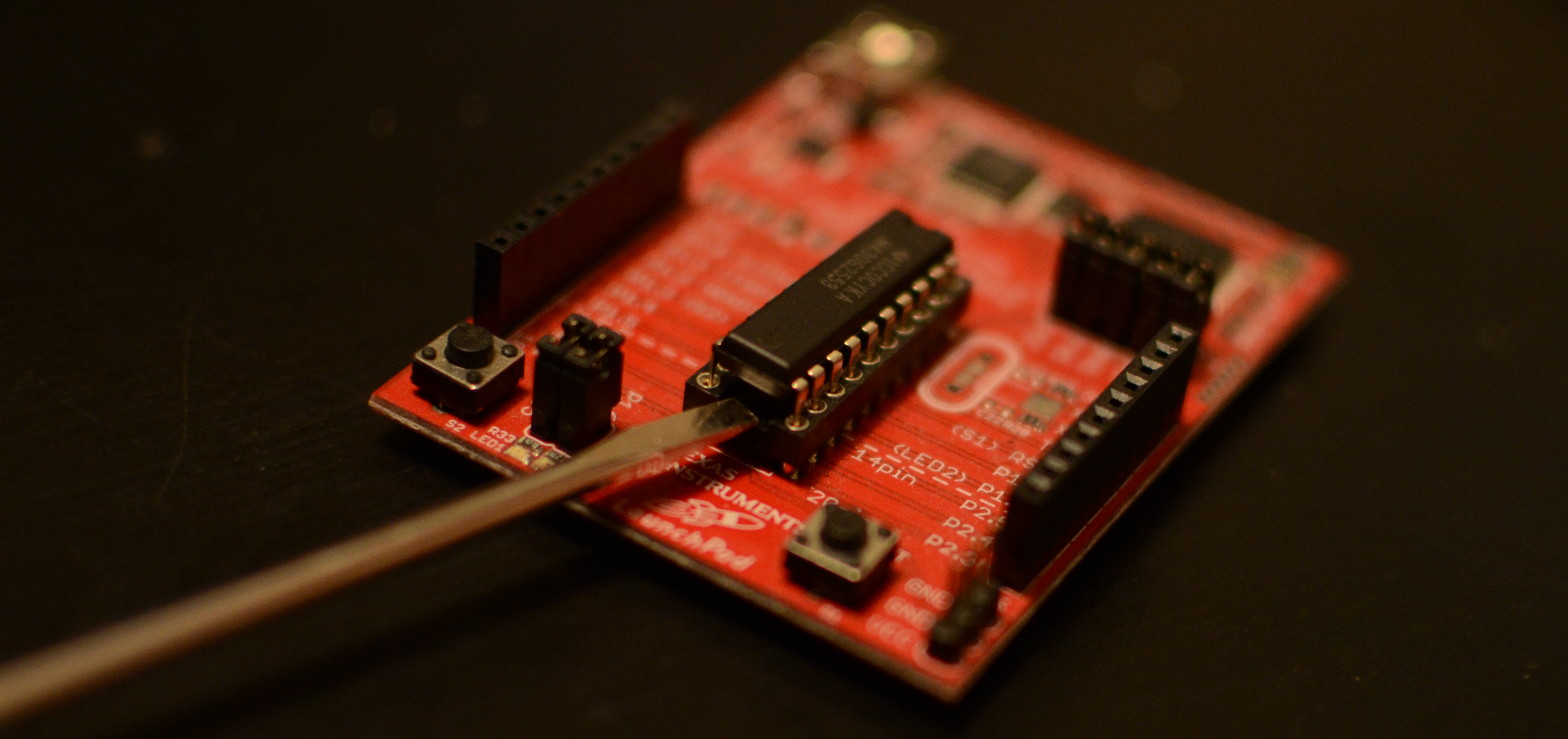
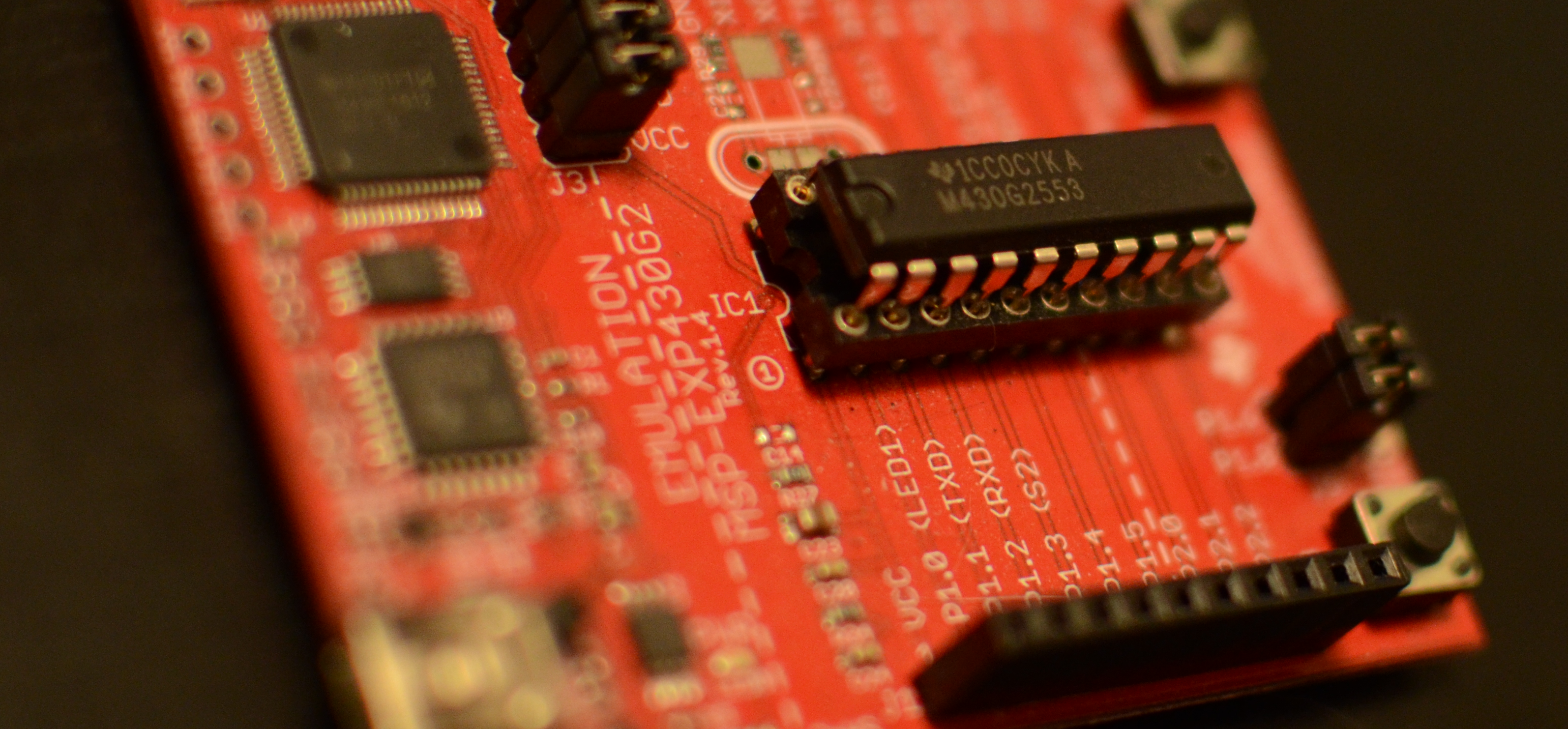
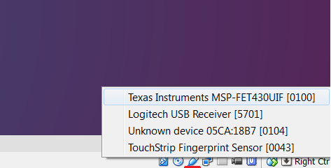

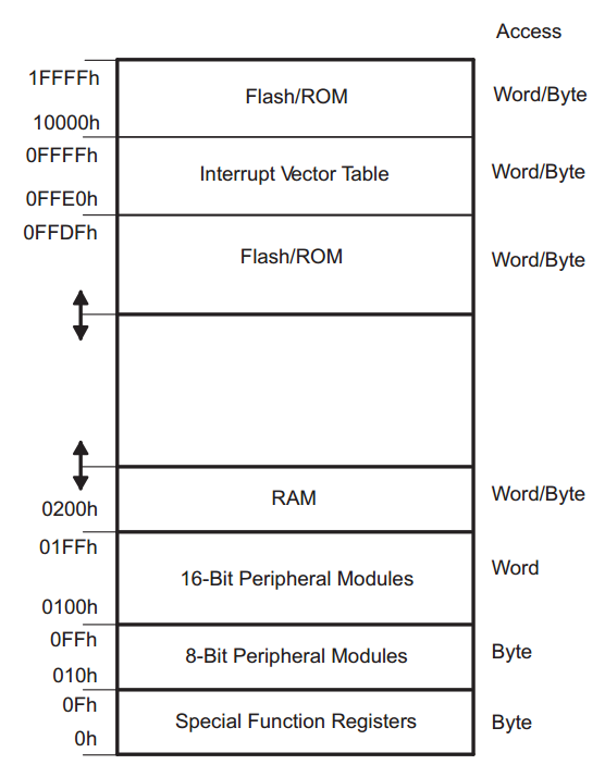
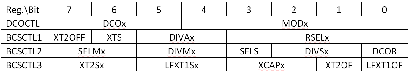

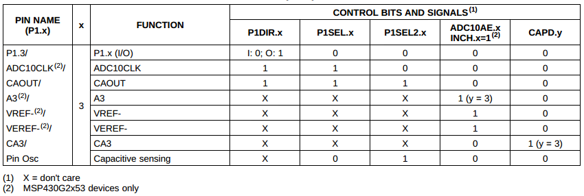
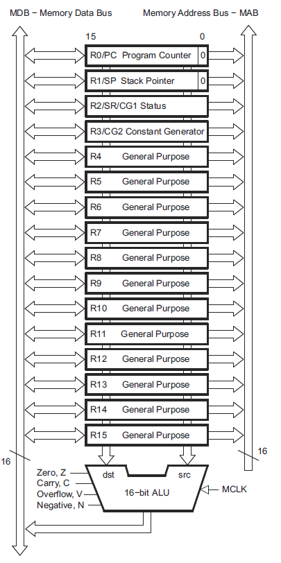
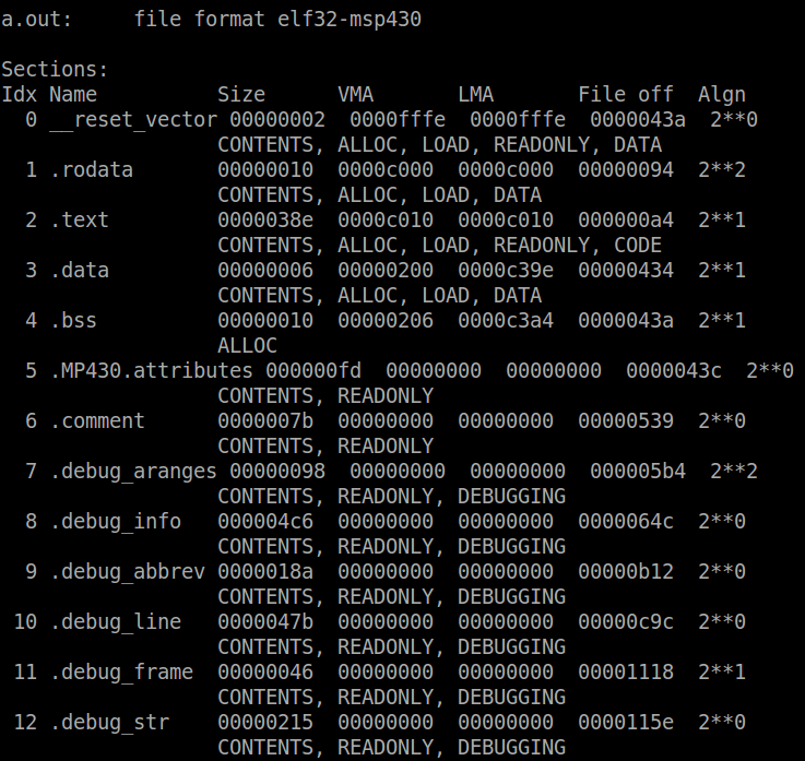
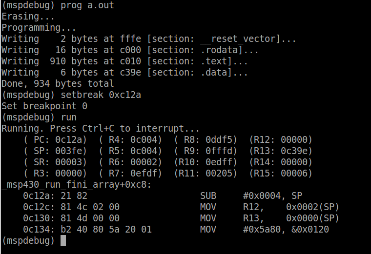
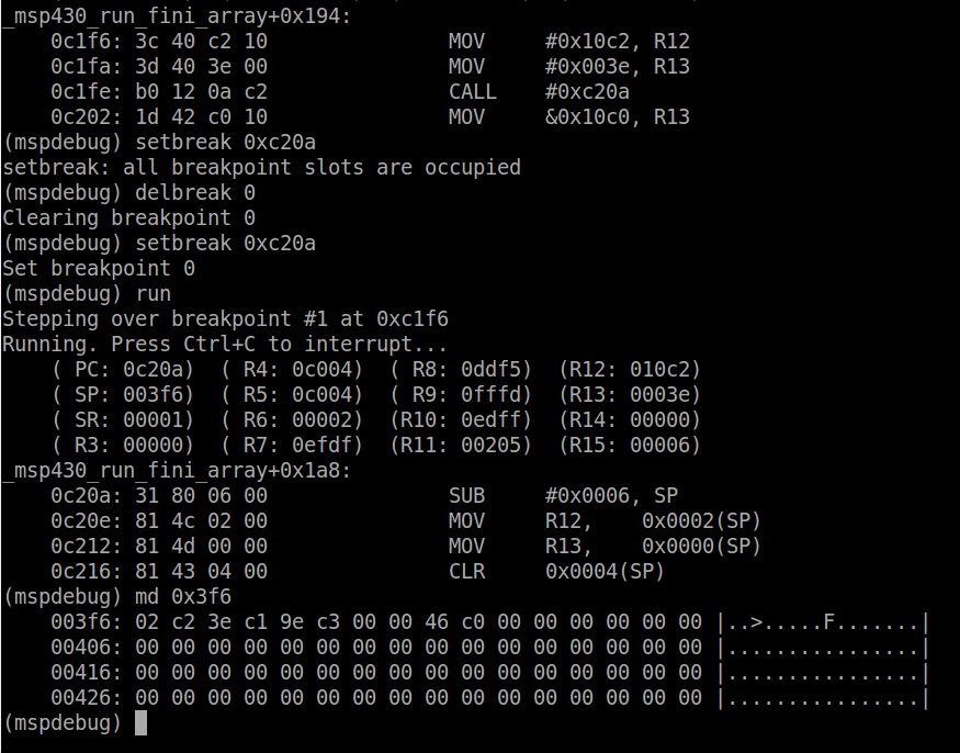

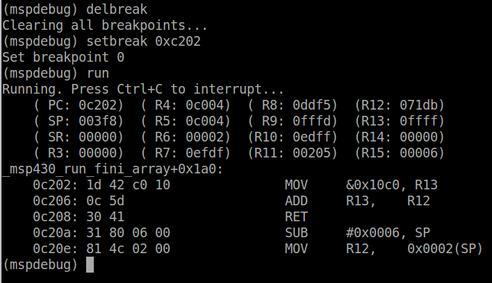

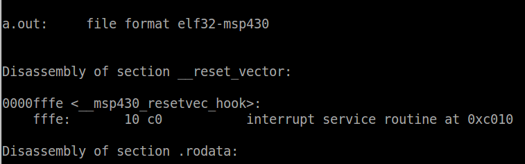

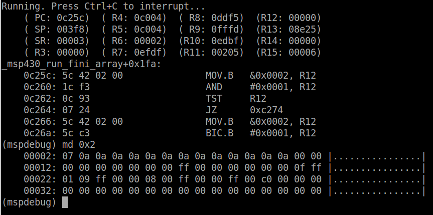
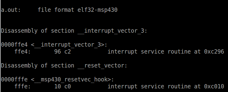
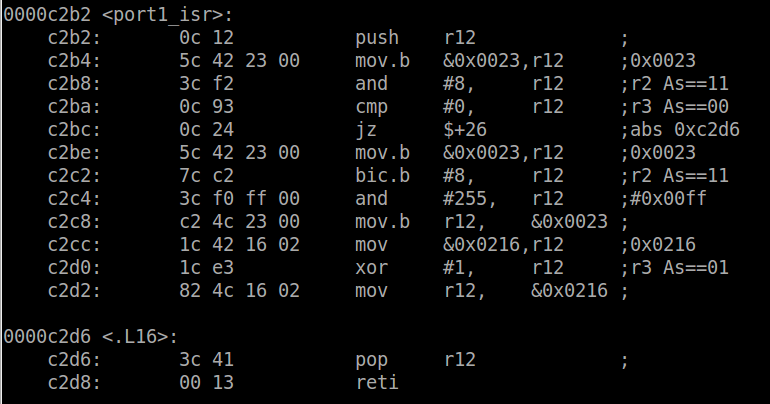
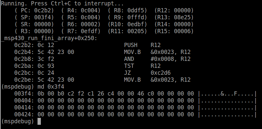

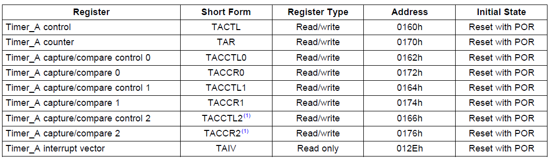
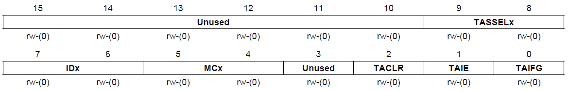
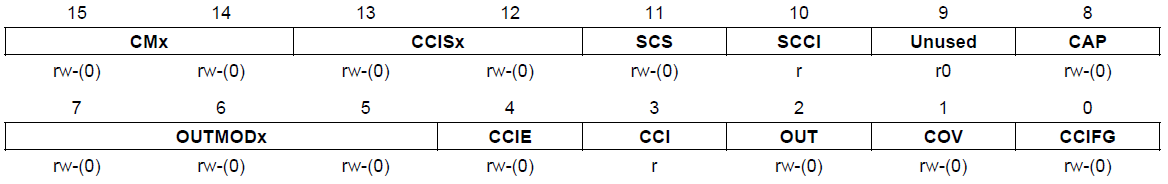
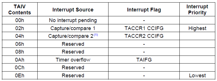
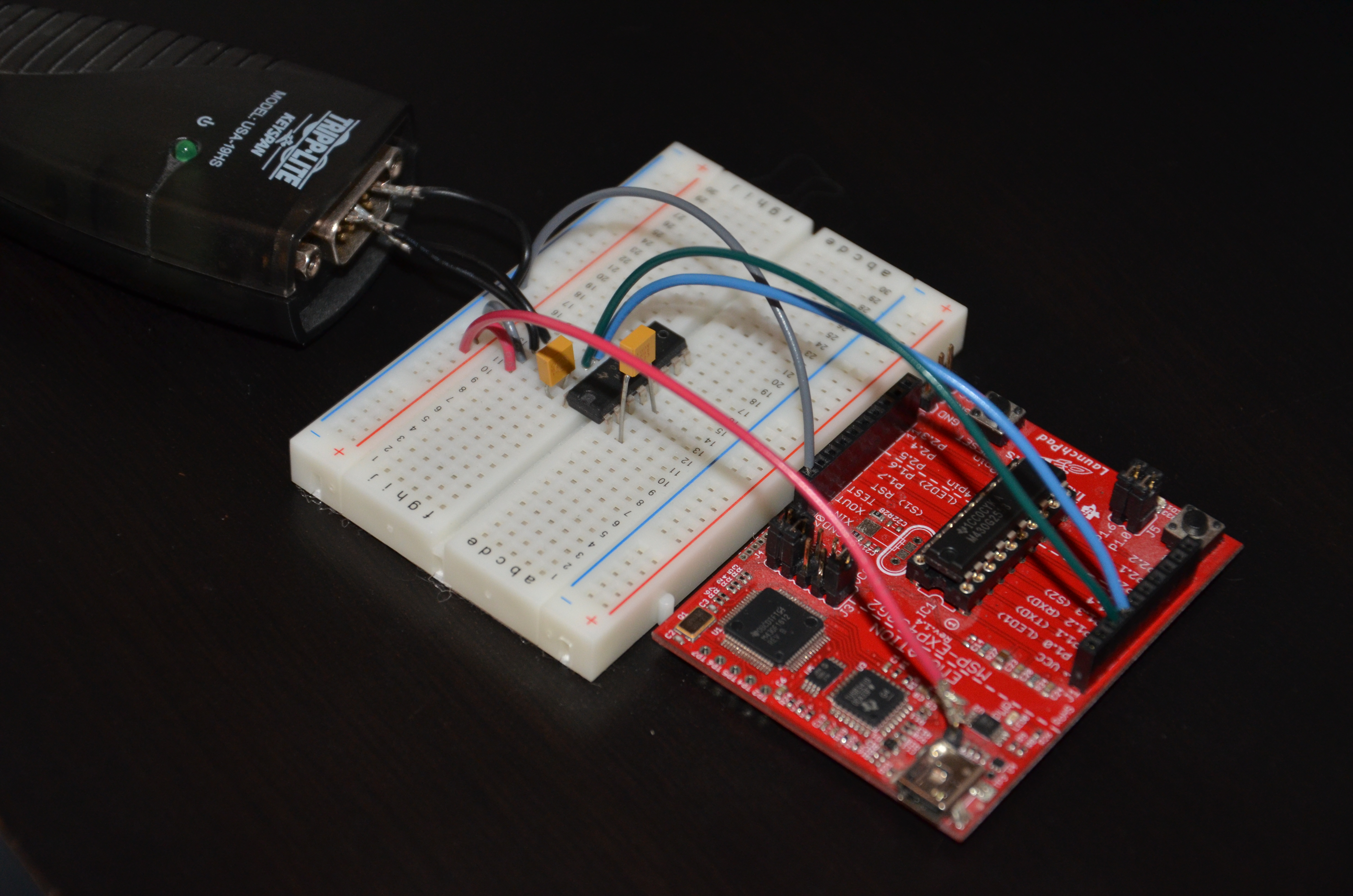
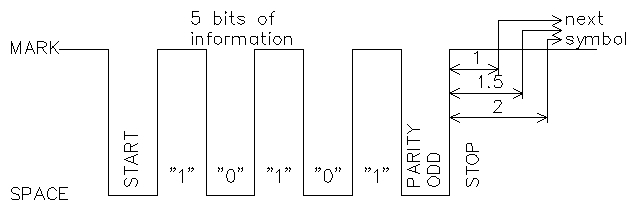
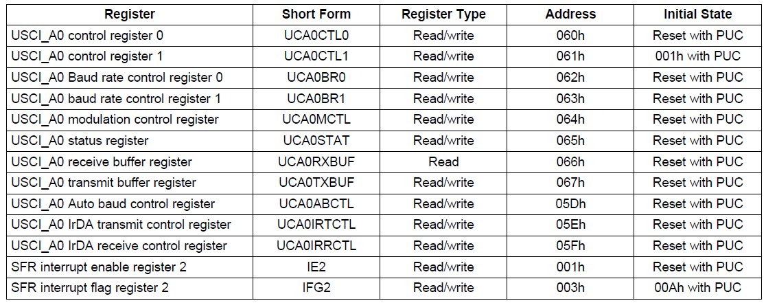


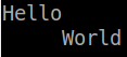


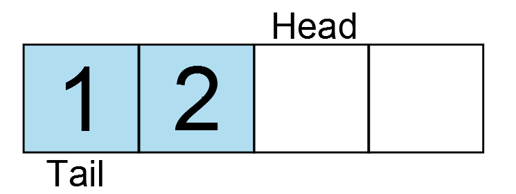
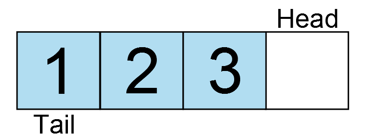
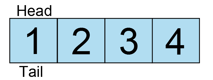
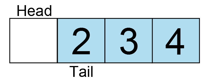
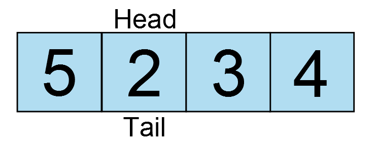

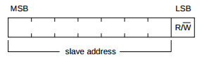
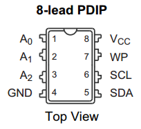
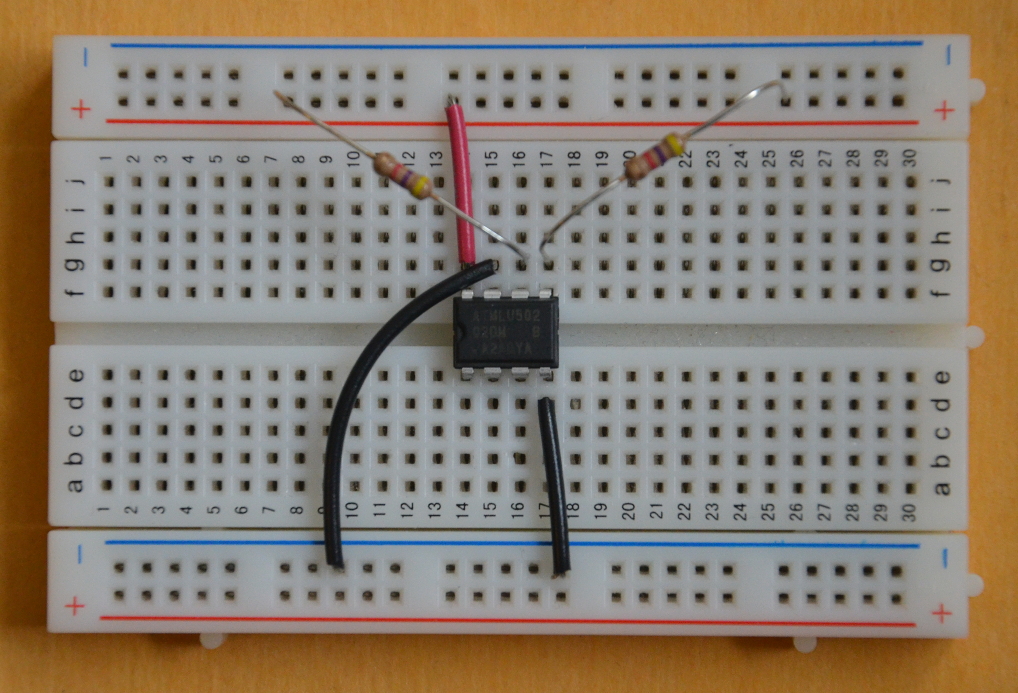

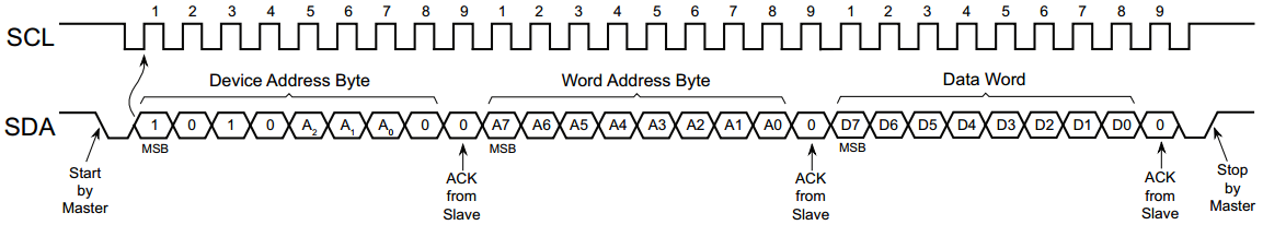
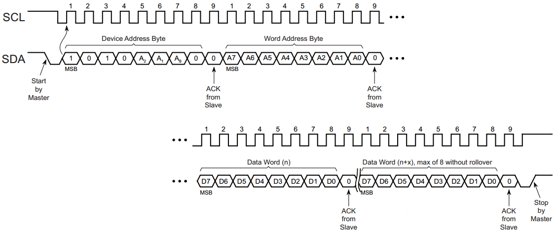
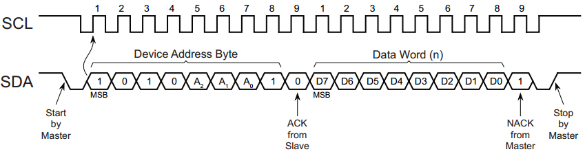
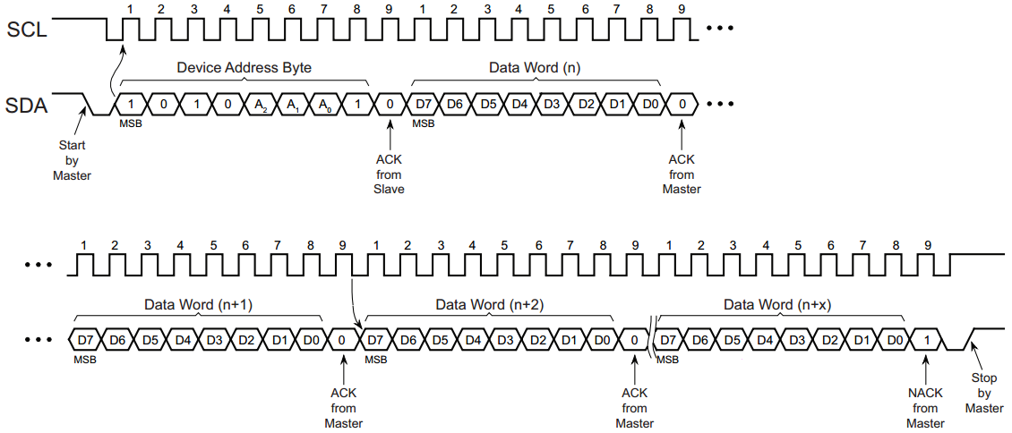


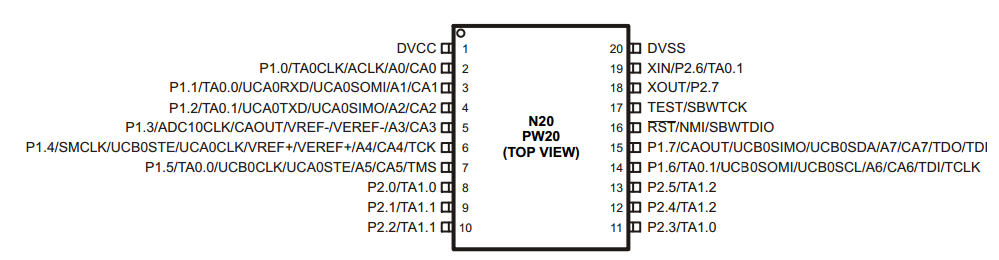
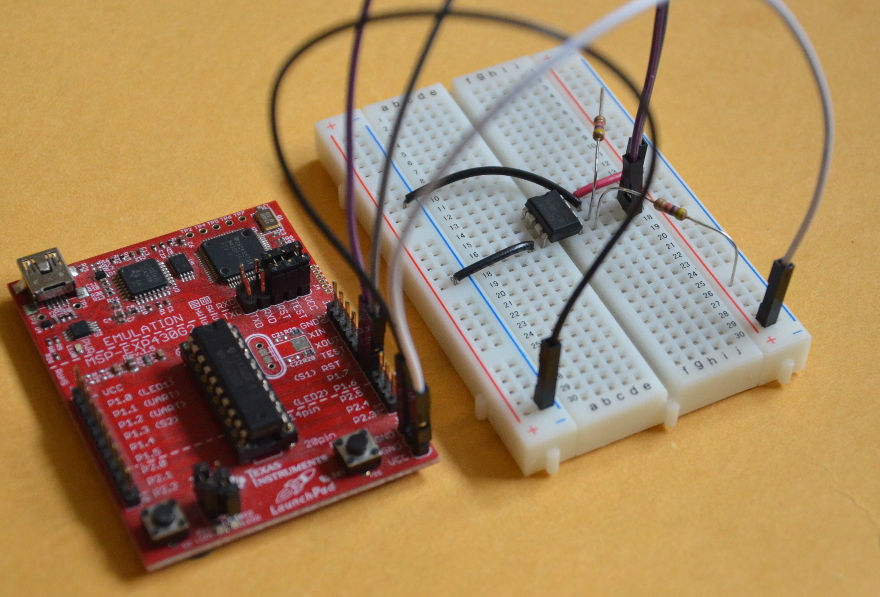
